Christopher Otrok and Charles H. Whiteman^*

version: September 28, 1996; printed 10/25/96

ABSTRACT

This paper designs and implements a Bayesian dynamic latent factor model for a vector of data describing the Iowa economy. Posterior distributions of parameters and the latent factor are analyzed by Markov Chain Monte Carlo methods, and coincident and leading indicators are given by posterior mean values of current and predictive distributions for the latent factor.

Keywords: Markov chain, Monte Carlo, index model, latent dynamic factor

We thank Robert Engle, John Geweke, Beth Ingram, Christopher Sims, James Stock, Ruey Tsay, and Mark Watson for helpful comments. Sid Chib graciously supplied us with GAUSS code for posterior analysis of regression models with autoregressive errors. Whiteman gratefully acknowledges the support provided for this research by the NSF under grant SBR 9422873.

I. Introduction

Where has the economy been? Where is it now? Where is it going? It is perhaps surprising that the latter of these three questions is not much more difficult to answer than the first two. Given historical data, econometric and time series techniques may be brought to bear on the forecasting problem. There are many alternative approaches to doing this, of course, but the issues associated with choice of methods and implementation of procedures are well understood. What is less well understood generally is that revisions to historical data are often substantial (so, where has the economy been?--if you dislike the current version of history, wait for the revision), and there are few generally accepted unidimensional measures of economic activity (where is the economy?--can you extract a simple signal from this morass of data?)

This paper addresses each of these two issues, and implements an indicator model for a vector of data describing the Iowa economy. The indicator is designed to be calculated monthly using data which are never or at least infrequently revised, and to provide a univariate measure of current economic conditions as well as a forecast of economic conditions six to nine months ahead. The current value of the factor is the "coincident" indicator of economic activity; a forecast of its value (say) sixth months hence is the "leading" indicator.

The technical innovation of the paper is that the economic indicator problem is treated as a (dynamic) latent factor problem. Using a Bayesian approach employing distributional assumptions typically used in economic forecasting, it is relatively straightforward to construct artificial "observations" on the unobservable indicator via data augmentation (Tanner and Wong, 1987). Markov chain Monte Carlo methods are used to sample from posterior distributions of the dynamic factor, and relevant quantiles and moments are calculated numerically.

The single factor formulation, while generalizeable, is motivated by the need for a simple measure of economic activity which can be quickly understood by business persons, policy makers, etc. The much more comprehensive Iowa Economic Forecast, published quarterly and used in planning exercises in a variety of ways in business as well as state government, comprises forecasts of about three dozen economic time series. These forecasts are generated using a Bayesian vector autoregression (BVAR) approach; see Whiteman (1996). Because entire predictive distributions are presented for a variety of relevant time series, the Forecast facilitates (and in fact advocates) use of non-quadratic and asymmetric loss functions. The highly multidimensional nature of the output of that exercise makes it useful for decision makers, but challenging to digest for more casual users. Indeed, policymakers and the media often press for a more prosaic summary of economic conditions and the forecast. While more numerical than prosaic, the unidimensional coincident and leading indicators meet this need.

II. The Single Factor Model

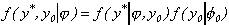
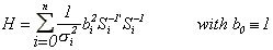
The model is patterned after the "new indexes of coincident and leading indicators" of Stock and Watson (1989, 1991). There are n variables, denoted y_i, i = 1,...,n, on which observations have been collected for periods t = 1, ... , T. There is a single common factor, y₀, which accounts for all comovement among the n variables. Thus

(1) y_it = a_i + b_iy_0t + e_it Ee_ite_jt-s = 0 for i j.

The idiosyncratic errors e_it may be serially correlated, and are modeled as p_i-order autoregressions:

(2) Eu_itu_jt-s = for i = j, s=0, 0 otherwise

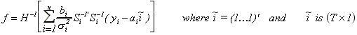
The evolution of the factor is likewise governed by an autoregression, of order q:

(3)

(4) Eu_0tu_0t-s = .

The innovations u_it, i = 0,...,n are assumed to be zero mean, normal random variables; i.e., u_it ~N(0,).

The system (1)-(4) constitutes an "unobservable index model" (Geweke, 1977; Sargent and Sims, 1977). Sargent and Sims argue that this structure captures in a rigorous way what Burns and Mitchell (1946) had in mind; it is a dynamic version of the factor model popular in other social sciences. Here, all intertemporal cross-correlation among the variables is accounted for by the dynamic factor. The model can be thought of as a generalization of the "variance-components" model, in which the components account not just for a contemporaneous covariance matrix of the observables, but for the entire spectral density matrix of y_it, i = 1,...,n. One feature of the model is that the sign of the dynamic factor and the sign of the b_i are not separately identified. This is handled by requiring one of the factor loadings to be positive.

If, contrary to assumption, the dynamic factor y_0t were observable, analysis of the system would be straightforward. Since it is not, special methods must be employed. Stock and Watson (1989, 1992, 1993) treat the model as an observer system and employ classical statistical techniques employing the Kalman filter/smoother to estimate the model parameters and extract an estimate of the unobserved factor. An alternative procedure can be based on a recent development in the Bayesian literature on missing data problems, that of "data augmentation" (Tanner and Wong, 1987.) The essential idea is to determine posterior distributions for all unknown parameters conditional on the latent factor, and then if the conditional distribution of the latent factor given the observables and the other parameters is available, the joint posterior distribution for the unknown parameters and the unobserved factor can be sampled by using a Markov Chain Monte Carlo procedure on the full set of conditional distributions.

Thus denoting by the set of parameters (b_i, , _i,j, i = 1,...,n), and the factor by f, suppose the conditional posterior distributions are given by p(j|f) and p(f|j). Starting from a value f⁰ (which must be in the support of the posterior distribution of f) produce a drawing j¹ by sampling from p(j|f⁰); produce f¹ by sampling from p(f|j¹), and so on. Under regularity conditions (see Geweke, 1995a, 1995b; Tierney, 1991, 1994; Chib and Greenberg, 1996), this produces a realization of a Markov chain whose invariant distribution is the joint posterior of interest.

In the present context, since conditional on the dynamic factor the equations in (1) are simply regression models with AR errors, the conditional posterior p(|f) is straightforward to analyze using the procedure due to Chib and Greenberg (1994). In fact, sampling from the conditional posterior simply requires n applications of the Chib-Greenberg procedure, which is already a Markov chain procedure. (One additional Chib-Greenberg pass is used to sample from the conditional posterior for the AR coefficients _0,j, j = 1,...,q.) What remains then is determination and analysis of the conditional posterior p(f|j). This is analogous to the customary "signal extraction" problem, except what must be extracted is not just the conditional mean, but the entire distribution. We proceed in two steps: first, we describe analysis of the posterior of j conditional on the factor; we then turn to the conditional distribution of the factor given j.

II.1. Conditional Distributions of Parameters Given the Factor

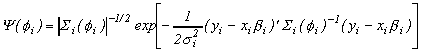
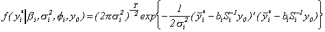
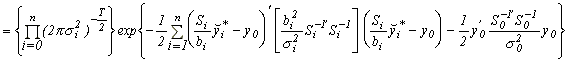
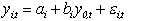
Given the factor y_0t, equations in (1) are simply n independent regression equations, each with autoregressive errors. Following Chib and Greenberg (1994), we build the posterior for the parameters by first determining the likelihood for the first p_i observations, sequentially conditioning to build the rest of the likelihood, and multiplying by the prior distribution. To begin, define

for i = 1,...,n. Thus variables with tildes denote the first p_i observations. The conditional mean of is straightforward, but the covariance matrix requires some work. Let

,

i.e., the companion matrix associated with the autoregression in (2). Then the covariance matrix of the first p_i errors is

or in vectorized form,

.

Then, as in Chib and Greenberg, the density of the first p_i observations on y_i is given by

(5)

To build the rest of the likelihood, first compute the Cholesky factor of S_i

and define

.

Then with the usual (conjugate) prior densities given by

where N_s is the s-variate Normal Distribution, and IG is the inverted gamma distribution, the conditional posterior distributions are given by (see Chib and Greenberg, 1994):

(6)

(7)

(8)

where

,

= indicator function for stationarity

It is straightforward to sample from the conditional distributions for b_i and . Sampling from the conditional distribution of _i is not because the kernel density is the product of a normal and the factor . Following Chib and Greenberg (1994), we sample from the distribution of _i using a Metropolis-Hastings algorithm. That is, at each iteration k, we generate a "candidate" from the distribution. Then = with probability = 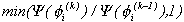and = with probability 1-. Chib and Greenberg (1994) establish convergence of this Markov chain procedure for sampling from the conditional distributions (6)-(8).

II.2. Conditional Distributions of Factor Given the Parameters

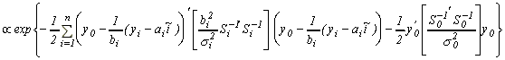
What we add in this paper is the remaining conditional distribution of the dynamic factor given the parameters whose conditional distributions were given in the previous subsection. To do this, we rebuild the likelihood function by multiplying the likelihood conditional on the factor by the marginal likelihood for the factor itself. Then, employing standard Normal conditioning arguments we derive the conditional distribution of the dynamic factor.

Define

where and compute all T "quasi-differenced" observations

Now let and note that the likelihood for the data conditioned on the factor is

for i = 1,...,n. Then the likelihood for the observables is

where . The marginal likelihood of the factor is:

.

Therefore, the full likelihood is

.

.

Since we are conditioning on parameters, the leading term is merely an integrating constant, and we have

.

Upon completing the square, we obtain

.

Therefore, the conditional distribution of the factor is recognized to be normal,

(9)

where

.

The difficulty with sampling from the conditional distribution of the factor arises because of the presence of the inverse of the TxT matrix H. This is the same problem which arises in the treatment of moving average errors, and arises for the same reason: the factor structure of the model gives the system an ARMA structure. What is fortunate is that the moving average component is common across the equations for the observables, and instead of n TxT inversions, only one is required.

II.3. Predictive Distributions of Factor Given the Parameters

The predictive distribution of the factor is found by sampling from the joint predictive density for all the observables and the factor. This requires drawing from the predictive (conditional on the factor and current draws of the AR coefficients and innovation variances) for each observable at each iteration of the Markov chain, and then sampling from the distribution of the factor given the actual data, the most recent sampled parameter values, and values from the predictive for the observables.

III. Implementation on Artificial Data

To gain insight into the facility with which the procedure recovers the unobserved factor, we initially experimented with an artificial system. The system consisted of four observables,

and the errors were AR(3) processes:

.

As above, the dynamic factor was given by

which was also AR(3):

.

The model parameters were given by

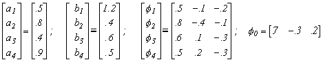
and the innovation distributions were

.

The initial were set equal to 0. Using draws from the above distributions for u_i , time series of length 500 were generated using the model equations and parameters above. The last 100 observations of the time series were saved and used in the simulations. The Markov chain procedure utilized 10000 replications after discarding 500 drawings from a "burn in" phase, and required about 320 minutes of P-5/90 Mhz CPU time.

Figure 1 displays a representative time series of two of the observables together with the hidden factor. Clearly there is a common signal to extract, but the signal to noise ratio is not so large as to make the exercise trivial.

The factor innovation variance was normalized by setting the variance equal to the average innovation variance from AR(q) autoregressions of the four observable series. The prior distributions for the a_i and b_i were:

The priors on the 's were:

The parameters for the inverted gamma distribution were both set equal to 0.

Table 1 reports posterior statistics for the parameters together with population values, and indicates that the procedure recovers parametric information quite well. Figure 2, which gives the 33%, 50% and 66% quantiles of the factor posterior distribution, illustrates how well the procedure performs in recovering the dynamic factor itself. The posterior distribution is somewhat disperse, but upon calculating the mean (across the 10000 replications) at each date and associated standard errors (of the posterior mean), the standard error bands are quite tight. In fact, the 2 standard error bands are indistinguishable from the mean. Figure 3 indicates as much; the process is seen to perform remarkably well in extracting the signal from the noise. We therefore proceed to implement the scheme on data from Iowa.

IV. A Dynamic Factor Model for Iowa

One potential difficulty in estimating a dynamic factor from state data is that the comovement in national variables is not so apparent in state data, even with analogous series. For example, Figure 4 displays four series selected for the observables in the Iowa factor model, together with their national counterparts. The series are: the midwest manufacturing index, average hourly earnings in manufacturing, average weekly hours in manufacturing, and total nonagricultural employment. These series, which are constructed primarily from establishment surveys, are infrequently revised, and are representative of series used in national economic indicators. The data are monthly and run from 1984:7 to 1995:8. There are very strong seasonal factors in these series, and as a consequence, attention is focused on year-over-year growth rates. In addition, month-to-month changes in year-over-year growth rates are of interest, so the observable data are first logged, then twelfth differenced, then first differenced to produce the series indicated in Figure 5.

The Iowa factor model was implemented under the same normalization and prior used to analyze the artificial data, and with p_i = 3, i = 1,...,4, q = 6. Also, 11 seasonal dummies were incorporated into each of the equations in (1) of the model; each seasonal dummy coefficient was given the same prior distribution as the constant.

The resulting posterior distributions are characterized in Table 2. (The normalization was that the factor loading on nonagricultural employment was positive.) Note that with the possible exception of manufacturing average hourly earnings, all factor loadings are significantly positive: a positive innovation to the factor indicates an increase in the year-over-year growth rate in the level of each series.

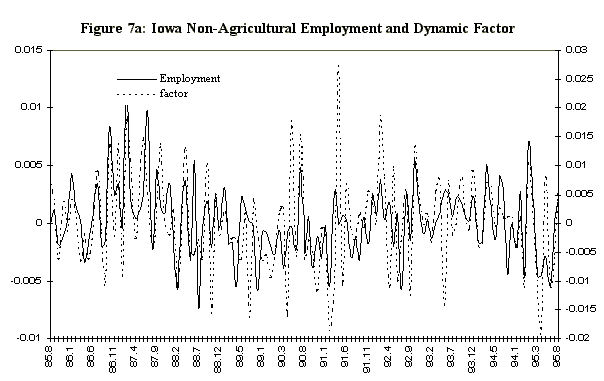
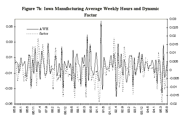
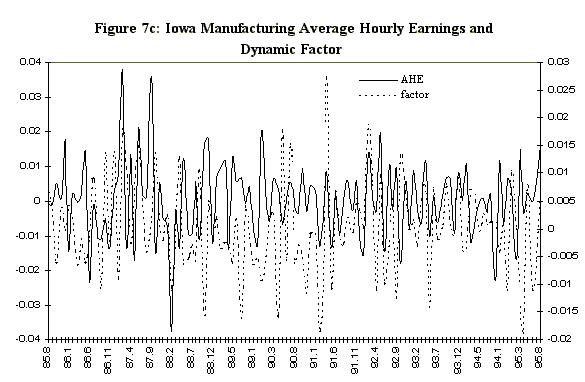
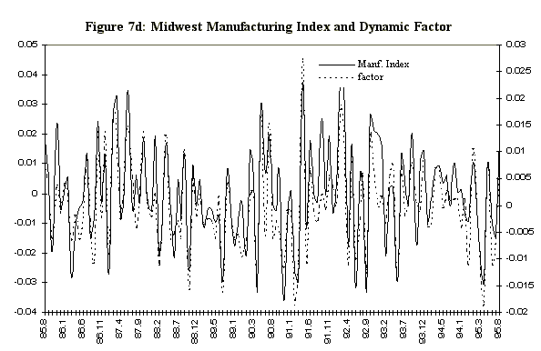
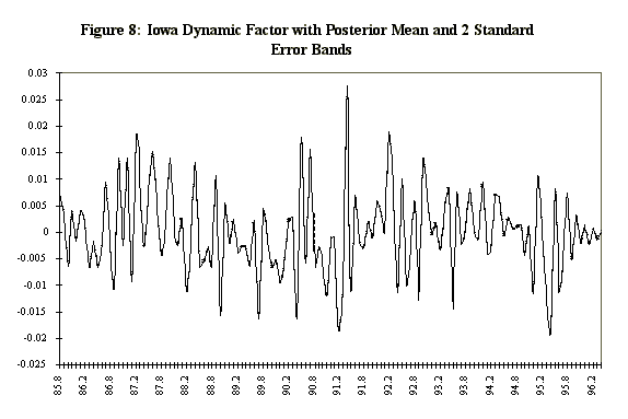
Figure 6 displays the 33%, 50%, and 66% quantiles of the in-sample posterior distribution of the Iowa factor, together with same quantiles of the predictive for the ensuing eight months. Since the factor in Figure 6 is very volatile a smoothed version of the factor is also estimated. The smoothed version (Figure 6b) is a 3 month moving average of the factor. The moving average is calculated at each step of the Markov chain so we have the entire distribution of the smoothed factor. Figure 7 displays the mean of the Iowa factor together with the Iowa data used in its construction, and emphasizes how the factor is picking up the comovement in the series. Figure 8 shows the mean and the associated standard errors of the means at each point in time. As with the artificial data the factor mean is indistinguishable from the standard error bands.

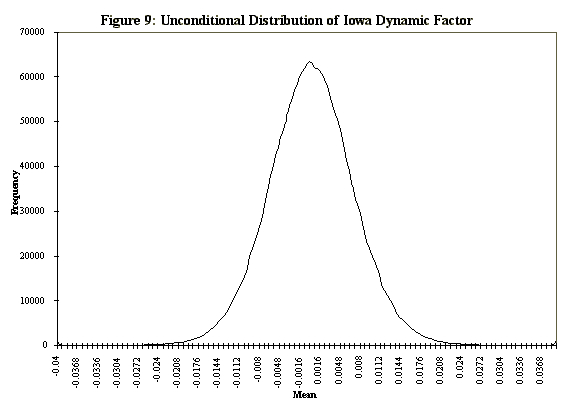
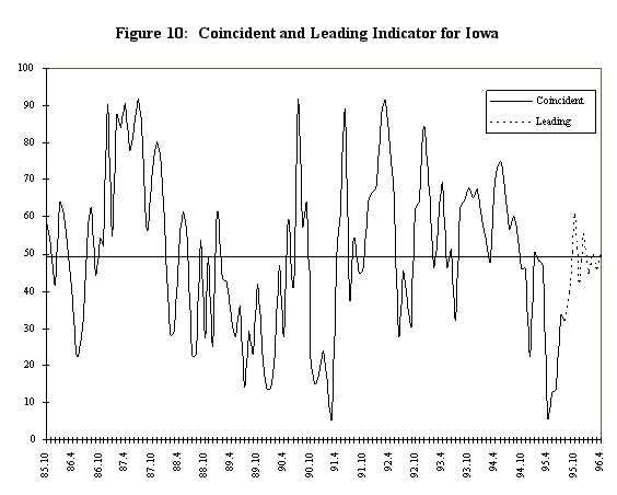
The actual index is constructed using the mean of the smoothed version of the factor at each date (including the forecast dates). These mean values are compared to the unconditional (across time) posterior distribution of factor means (Figure 9). The quantile of the unconditional distribution at which the mean for each date falls is calculated and reported as the index. For example, at the end of the sample, the posterior mean of the smoothed Iowa factor for 1995:8 is -.003, which is the 32nd quantile of the unconditional distribution, so the value of the coincident indicator is 32. What this signifies is that the 1 month change in the year-over-year growth for the 3 months ending in August in the Iowa economy was well below average.

The leading indicator is calculated similarly. For example, the predictive mean of the factor for 1996:3 is -.0007, which falls in the 46th quantile of the unconditional distribution, leading to a value of the leading indicator of 46, indicating monthly change in the year-over-year growth in the first 3 months of 1996 will be slightly below average.

VI. Conclusion

This paper has provided a Bayesian approach to the calculation of coincident and leading economic indicators. The principal contribution is the derivation of the conditional distribution of the dynamic factor in an "unobservable index model" which can be used together with previous results due to Chib and Greenberg (1994) and Markov chain methods to facilitate numerical analysis of the joint posterior distribution of parameters and the unobserved factor. The scheme was illustrated on artificial data, and implemented to construct a coincident and leading indicator for the Iowa economy.

Burns, Arthur F. and Wesley C. Mitchell (1946), Measuring Business Cycles. New York: National Bureau of Economic Research.

Chib, Siddhartha and Edward Greenberg (1994), "Bayes Inference in Regression Models with ARMA (p,q) Errors," Journal of Econometrics, 64:183-206.

Chib, Siddhartha and Edward Greenberg (1995),"Understanding the Metropolis-Hastings Algorithm," American Statistician 49 (November):327-335.

Chib, Siddhartha and Edward Greenberg (1996),"Markov Chain Monte Carlo Simulation Methods in Econometrics," Econometric Theory 12:409-431.

Geweke, John (1977), "The Dynamic Factor Analysis of Economic Time Series," in D. J. Aigner and A. S. Goldberger eds. Latent Variables in Socio-Economic Models, Amsterdam: North Holland Publishing, Chapter 19.

Geweke, John (1995a), "Monte Carlo Simulation and Numerical Integration," Handbook of Computational Economics, forthcoming.

Geweke, John (1995b), "Posterior Simulators in Econometrics," Federal Reserve Bank of Minneapolis working paper.

Iowa Economic Forecast, quarterly 1990:I - present. Iowa City: Institute for Economic Research.

Sargent, Thomas J. and Christopher A. Sims (1977), "Business Cycle Modeling Without Pretending to Have Too Much A Priori Economic Theory," in Christopher A. Sims et al., New Methods in Business Cycle Research, Minneapolis: Federal Reserve Bank of Minneapolis.

Stock, James H. and Mark W. Watson (1989), "New Indexes of Coincident and Leading Economic Indicators," NBER Macroeconomics Annual 1989, The MIT Press, pp. 351-394.

Stock, James H. and Mark W. Watson (1992), "A Procedure for Predicting Recessions with Leading Indicators: Econometric Issues and Recent Performance," Federal Reserve Bank of Chicago Working Paper, WP-92-7.

Stock, James H. and Mark W. Watson (1993), "A Procedure for Predicting Recessions with Leading Indicators: Econometric Issues and Recent Experience," in James H. Stock and Mark W. Watson eds. Business Cycles, Indicators, and Forecasting, The University of Chicago Press, pp 95-153.

Tanner, M., and W. H. Wong, 1987, "The Calculation of Posterior Distributions by Data Augmentation," Journal of the American Statistical Association 82:84-88.

Whiteman, C. H., 1996, "Bayesian Prediction Under Asymmetric Linear Loss: Forecasting State Tax Revenues in Iowa," forthcoming, Bayesian Inference in Statistics and Econometrics: Essays in Honor of Seymour Geisser. Berlin: Springer-Verlag.

Table 1: Population Values and Posterior Moments of Parameters in Artificial Data Dynamic Factor Model
	pop		posterior			pop.				posterior
parameter	value	mean	stnd dev	median	parameter	value		mean		stnd dev		median
a1	.5	.320	.595	.318		.5		.628		.182		.646
a2	.8	1.079	.330	1.072		-.1		-.314		.202		-.326
a3	.4	.320	.371	.321		-.2		.114		.154		.123
a4	.9	.485	.359	.485		.8		.667		.159		.674
b1	1.2	.338	.154	.332		-.4		-.290		.194		-.299
b2	.4	.202	.105	.200		-.1		-.080		.149		-.074
b3	.6	.409	.151	.418		.6		.362		.117		.363
b4	.5	.257	.104	.261		.1		-.015		.122		-.015
	3	7.412	1.421	7.300		-.3		-.333		.115		-.336
	4	4.014	.714	3.975		.5		.448		.108		.448
	9	9.324	1.794	9.171		.2		.121		.116		.122
	6	5.914	1.036	5.827		-.3		-.330		.107		-.330
	.7	.220	.218	.227
	-.3	-.048	.234	-.050
	.2	-.045	.242	-.050

Table 2: Posterior Moments of Parameters in Iowa Dynamic Factor Model
		posterior				posterior
parameter	mean	stnd dev	median	parameter	mean	stnd dev	median
a1	-.001	.006	-.001	S1,8	-.0006	.0079	-.0008
a2	.000	.004	.000	S1,9	-.0031	.0078	-.0031
a3	-.001	.005	.000	S1,10	.0011	.0077	.0010
a4	.001	.001	.001	S1,11	.0011	.0081	.0010
b1	.916	.241	.926	S2,1	.0008	.0061	.0008
b2	.050	.123	.049	S2,2	.0009	.0051	.0009
b3	.590	.231	.581	S2,3	.0002	.0056	.0003
b4	.110	.038	.111	S2,4	-.0010	.0054	-.0010
	.000178	.000046	.000175	S2,5	.0024	.0056	.0024
	.000130	.000018	.000128	S2,6	-.0005	.0054	-.0004
	.000147	.000029	.000146	S2,7	-.0003	.0056	-.0003
	.000009	.000002	.000009	S2,8	-.0005	.0054	-.0004
	-.085	.136	-.088	S2,9	-.0002	.0056	-.0002
	-.022	.133	-.021	S2,10	.0012	.0050	.0013
	.082	.138	.087	S2,11	-.0016	.0062	-.0016
	.010	.122	.009	S3,1	.0015	.0074	.0015
	.030	.101	.031	S3,2	-.0002	.0066	-.0003
	-.005	.075	-.005	S3,3	.0017	.0071	.0016
	-.085	.136	-.088	S3,4	-.0003	.0065	-.0004
	-.022	.133	-.021	S3,5	-.0008	.0070	-.0008
	.082	.138	.087	S3,6	.0009	.0066	.0008
	-.257	.100	-.257	S3,7	.0023	.0070	.0022
	.103	.102	.103	S3,8	.0000	.0064	.0000
	.040	.099	.040	S3,9	-.0022	.0071	-.0022
	-.345	.171	-.353	S3,10	.0009	.0067	.0009
	-.158	.151	-.162	S3,11	.0010	.0075	.0010
	-.126	.129	-.132	S4,1	-.0011	.0015	-.0011
	-.082	.107	-.081	S4,2	-.0008	.0014	-.0008
	.145	.108	.148	S4,3	.0000	.0016	.0000
	.010	.109	.008	S4,4	.0001	.0015	.0001
S1,1	.0031	.0079	.0031	S4,5	-.0004	.0015	-.0004
S1,2	.0014	.0079	.0014	S4,6	.0003	.0015	.0003
S1,3	.0002	.0077	.0001	S4,7	-.0002	.0016	-.0002
S1,4	.0034	.0078	.0033	S4,8	-.0004	.0015	-.0004
S1,5	.0012	.0081	.0011	S4,9	-.0012	.0016	-.0011
S1,6	.0004	.0076	.0004	S4,10	-.0009	.0014	-.0009
S1,7	.0122	.0079	.0012	S4,11	.0004	.0016	.0004

Note: S_i,j is the coefficient on the jth seasonal dummy in the ith observable equation. Variable 1 is

the midwest manufacturing index, variable 2 is manufacturing average hourly earnings,

variable 3 is manufacturing average weekly hours and variable 4 non-agricultural employment.

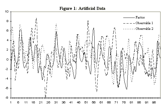
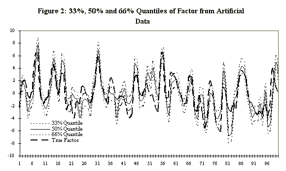
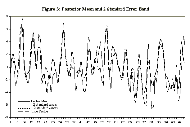
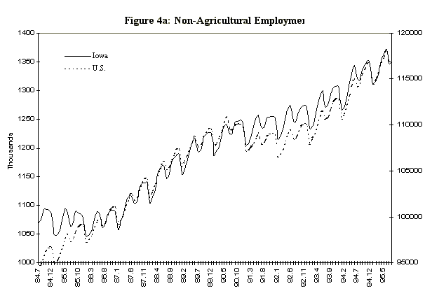
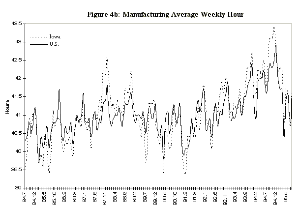
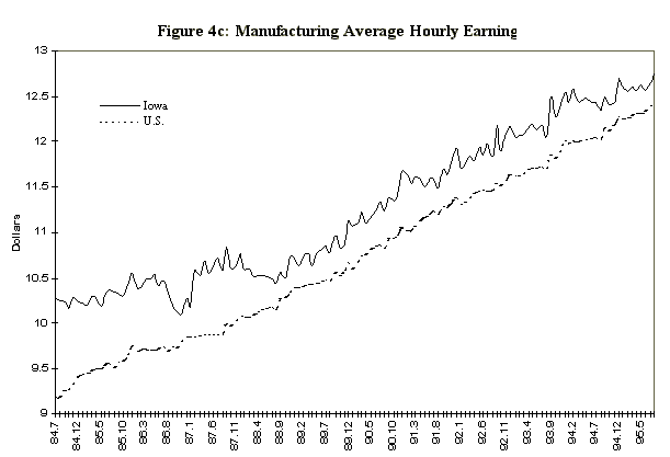
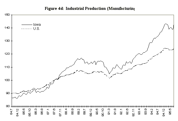
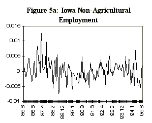
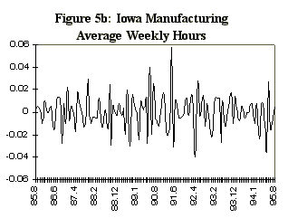
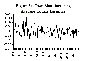
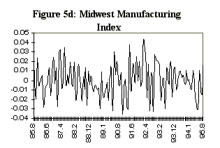
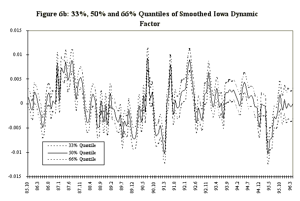Figure 7: Iowa Data and Dynamic Factor