Rodney D. Ludema
Department of Economics
Georgetown University
Washington DC 20057, USA
Ian Wooton
Department of Economics
University of Glasgow
Glasgow G12 8RT, UK
Centre for Economic Policy Research
45-48 Old Burlington Street
London W1X 1LX, UK
Abstract
We examine the consequences of increased economic integration between nations within a region. We adopt Krugman’s economic-geography model in which demand linkages can generate agglomeration of manufacturing activity. Manufacturing labour is assumed to be imperfectly mobile between countries. This constrains the forces of agglomeration within the region and suggests that the model may be applicable to Europe. We show that trade liberalisation may lead initially to partial agglomeration, then a re-industrialisation of the periphery. This argues in favour of a sequential approach to integration, with trade barriers being eliminated prior to a reduction in impediments to factor mobility.
Keywords: economic integration, economic geography, factor mobility, international trade
JEL codes: F12, F15, F22
January 1997
Second Revision, July 1997
1. Introduction
In this paper we examine the consequences of increased economic integration between nations within a region. We assume that the countries already have made significant strides towards a common market by lowering trade costs and impediments to factor mobility. However, some barriers remain and we shall consider economic integration as a combination of dropping barriers to factor mobility and reducing transport costs. We are interested in determining the circumstances under which economic integration will lead to agglomeration of economic activity, whereby one part of the region will accumulate virtually all of the manufacturing activity, while the remainder will become largely de-industrialised. This clearly is an important issue for a regional grouping such as the European Union (EU), particularly given its recent efforts to deepen the level of integration between member states.
We adopt the general-equilibrium, economic-geography model of Krugman (1991a) to characterise what we refer to as the "labour-demand" side of the model. This produces the agglomerative forces that can lead to a core-periphery pattern through backward and forward "demand linkages". The backward linkage captures the notion that manufacturing production will tend to concentrate where there is a large market, but that the market will be large where manufacturing production is concentrated (because this is where the manufacturing workers live and consume). This is reinforced by the forward linkage in which, other things equal, the cost of living will be lower in the country with the larger manufacturing sector, because consumers in that location can rely less on imports (which are subject to transport costs). Both of these linkages will tend to draw manufacturing workers into the core, leaving the remainder of the region a rural hinterland.
In addition to the barriers to trade in manufactures, we allow for the imperfect mobility of manufacturing labour, which results in an upward-sloping international labour-supply schedule. Thus workers are assumed to have preferences for living in a particular country and, in order to induce them to migrate, a relatively higher real wage will have to be offered in the other country. We believe this to be a useful innovation for economic geography models applied to regions in which language and cultural barriers are significant, despite the lack of formal, legal impediments to mobility.
The benefits of introducing of imperfect labour mobility into this framework are more than merely adding realism. First, it substantially expands the possible outcomes arising from economic integration. Depending on the relative importance of agglomerative forces and labour mobility, integration may have no impact on the location of manufacturing activity or it may drive it to complete agglomeration, as in Krugman (1991a). An intermediate and more interesting possibility is that integration, in form of the progressive reduction of trade barriers, may be accompanied by a three-stage pattern of industrial production: international diversification, followed by the agglomeration of activity into core-periphery pattern, followed by the re-industrialisation of the periphery.
Second, introducing imperfect labour mobility allows us to examine the effects of a dual approach to integration, that of reducing trade barriers and reducing barriers to mobility. We show that it may be possible to eliminate temporary agglomeration, and its concomitant disruptions, by appropriately sequencing the two forms of integration.
Krugman (1991a) originally set out the demand linkages model, in part, to explain the core-periphery patterns of North America and Europe. However, Krugman (1991b) cites data suggesting that Europe’s core-periphery pattern is more of an income pattern than an employment pattern. That is, as compared to the US, Europe exhibits more pronounced differences in per-capita income across its constituent states, but less pronounced differences in the concentration of manufacturing labour. His conclusion is that the demand linkages model does not explain this. This is echoed by Venables (1994) who writes, "migration in Europe is perhaps insufficiently responsive to economic factors for [the demand linkage] mechanism to be of much relevance to European integration."
A second point mentioned in Krugman (1991b), as well as in Krugman and Venables (1995), is that there are signs of a gradual re-industrialisation of the periphery, in North America, Europe, and East Asia. Krugman and Venables (1995) use an alternative model, in which labour is internationally immobile (but intersectorally mobile), to generate a three-stage pattern similar to the one described above. They contrast this alternative model to the demand-linkage model as follows:
"Simple geography models like Krugman (1991a) respond in a monotone way to declining transport costs: when these costs fall below a critical level, industry concentrates in one region. Here, because labor is immobile (and thus wage differentials between regions emerge), continuing reductions in transport costs eventually lead to a reindustrialization of the low-wage region. We believe this is not just an artifact of the model: it represents a real distinction between interregional and international economics because labor is in fact much less mobile between than within nations."
All of this appears to cast doubt on the demand-linkage model, particularly in its application to Europe. However, it is our view that the results of the demand-linkage model that appear at odds with the facts are essentially artefacts of the assumption of perfect labour mobility. With the assumption of imperfect labour mobility (not complete immobility), we show that the experience of Europe is completely consistent with the demand-linkage model. It is entirely possible for a region like the US, because of its greater labour mobility (flatter labour-supply schedule), to exhibit more pronounced differences in employment and less pronounced differences in per capita income than Europe. It is also entirely possible to generate a three-stage integration pattern.
The layout of the paper is as follows. In section 2 we give the details of the structure of Krugman’s model, which provides the labour-demand schedule. We follow this, in section 3, by an examination of the influence of locational preference on labour supply. The resulting equilibria are discussed in section 4, while section 5 consists of some comparative statics exercises of more liberal trade and factor mobility. Section 6 concludes.
2. The Model
We model labour demand using Krugman’s (1991a) model of economic geography. This has two sectors: agriculture and manufacturing. Agriculture produces an homogeneous good according to constant returns to scale with farm labourers as the sole, sector-specific factor. A unit of the agricultural product requires the input of one labourer. The agricultural workers are internationally immobile. In contrast, the manufacturing industry produces differentiated products with increasing-returns-to-scale technology. It employs internationally mobile labour. Each variety of the manufactured good is produced with increasing returns, these scale economies leading to the concentration of production of each variety in a single plant.
The homogeneous agricultural commodity can be traded costlessly, while trade in the differentiated good involves iceberg-type trade costs. As a result, there may be a tendency for plants to locate in the country in which demand for the variety is greater, so as to minimise these trade costs. Thus the nominal wage may be higher in the larger country. In addition, the cost of living differs internationally as imported varieties attract trade costs. Workers therefore may have an incentive to move to the industrialised "core" where the real wage is higher than in the agricultural "periphery", and this concentration of workers increases the size of the market in the core and reinforcing the decisions of firms to locate there.
All individuals share the same Cobb-Douglas utility function:
![]() ( 1 )
( 1 )
where CA is consumption of the agricultural good and CM is consumption of the aggregate manufactured good. Therefore agents will always spend the proportion m on manufactures. The manufactures aggregate is defined by:
 ( 2 )
( 2 )
where N is the (large) number of potential products and s > 1 is the elasticity of substitution among the varieties.
There are two countries in the economic region and two sector-specific factors of production in each country. Agricultural workers are internationally immobile, the supply in each country being ![]() . Manufacturing workers may move between countries. Let L1 and L2 be the numbers of workers in country 1 and country 2, respectively, where:
. Manufacturing workers may move between countries. Let L1 and L2 be the numbers of workers in country 1 and country 2, respectively, where:
![]() ( 3 )
( 3 )
Production of a representative variety of the manufactured good produced in country i involves a fixed cost and a constant marginal cost:
![]() ( 4 )
( 4 )
where xi is output of that variety and LMi is the labour used in its production. Agricultural output is freely traded and hence agricultural workers’ earnings are the same in both countries and shall be our numeraire. For manufactures, a proportion t < 1 that is shipped from one country arrives in the other.
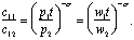
There is a large number of manufacturing firms, each producing a single product and facing an elasticity of demand equal to s . Profit maximising behaviour will lead firms to price their variety at a mark-up over marginal costs:
![]() ( 5 )
( 5 )
where wi is the wage rate of workers in country i. Relative prices must then be:
![]() ( 6 )
( 6 )
Free entry implies zero profits, hence:
![]() ( 7 )
( 7 )
which implies:
![]() ( 8 )
( 8 )
The numbers of varieties of the manufactured good produced in country i is ni. Combining equations (4) and (8) yields:
![]() ( 9 )
( 9 )
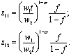
The quantities of each variety consumed will depend on their prices. Prices of imports must take into account the transport cost. Hence, for country 1,
 ( 10 )
where cij is the quantity consumed in country i of a variety manufactured in country j.
The share of the manufacturing labour force in country 1 is denoted ![]() . Define z11 to be the ratio of country 1’s expenditure on local products to its expenditure on varieties imported from country 2, while z12 is the ratio of country 2’s expenditure on manufactured imports to its expenditure on local goods. Therefore:
. Define z11 to be the ratio of country 1’s expenditure on local products to its expenditure on varieties imported from country 2, while z12 is the ratio of country 2’s expenditure on manufactured imports to its expenditure on local goods. Therefore:
The total income of workers equals the total spending on the products that they produce. If Yi is the national income of region i (including agricultural income), then the nominal wages of an individual worker in each region is:
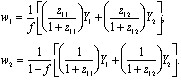 ( 12 )
where:
For a given allocation of manufacturing labour f, equations to are a system that determines nominal wages, incomes, and spending patterns.
Because of transport costs, the prices of manufactures differ in the two countries and therefore the cost of living will be a determinant of a worker’s decision as to location. The price indices of manufactured goods are:
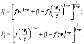 ( 14 )
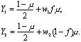
Real wages of workers in each country are:
 ( 15 )
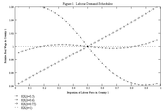
Figure 1 illustrates the labour-demand schedule KK, plotting f, the proportion of the (manufacturing) labour force in country 1, against w º w 1/w 2, the real wage in country 1 relative to that in country 2. Using an elasticity of substitution between manufactures s = 4, as in Krugman (1991a), the figure shows dramatic differences in the schedules for different trade costs. With high trade costs, the forces of agglomeration are low—when there are consumers in both locations, firms will produce in both countries. This is drawn as KK(t = 0.5). As trade costs fall, the stronger the agglomerative forces become, as illustrated by KK(t = 0.6) and KK(t = 0.75).
Figure 1 here.
It is worth noting that having even more liberal trade makes the KK curve flatter. Indeed, as t approaches one, the KK curve approaches horizontal. That the slope of the KK curve rises and then falls as the transport cost is reduced is largely irrelevant in the presence of perfect labour mobility (that is, as in Krugman, 1991a), but it turns out to be very important in the presence of imperfect labour mobility, as we shall see in section 5.
3. Labour Supply
Mobile workers are assumed to have different preferences over the location in which they would rather live and work. Because of these, the relative wage that will have to be offered to induce each worker to migrate will depend on the strength of her locational preference. We shall show that this can have a significant effect in mitigating the forces of industrial agglomeration that arise in the presence of increasing-returns-to-scale technology.
An industrial worker will make her decision as to where to live and work based on a comparison of real wages, in the light of her strength of preferences for living in each country. Why a worker prefers one country or the other is not explicitly modelled, merely being represented as a discount rate that would have to be applied to the relative real wage in order to induce the worker to move. However, real-world experience certainly provides a great deal of casual evidence of non-pecuniary benefits that individuals enjoy from living in one country or the other. These preferences will be represented by a density function and we shall examine how changes in the distribution may alter the structure of industrial production within the region.
Let g i be worker i’s discounting of the real wage offered in country 1, while (1 - g i) is her discounting of the real wage in country 2. Worker i will be indifferent between the two locations when the discounted real wages are equalised, that is:
We assume that workers’ preferences are distributed normally across the interval [0, 1]. Let the density of g i be given by:
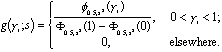 ( 17 )
where ![]() is a normal distribution with mean 0.5 and standard deviation s > 0, and
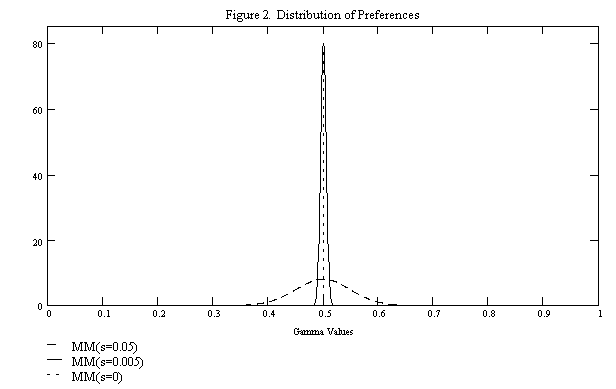
is a normal distribution with mean 0.5 and standard deviation s > 0, and ![]() is a normal density. By adopting this distribution and mean of 0.5, we are assuming that workers are on average indifferent between the two locations, and that deviations from indifference are symmetric. The greater is s, the stronger the location preferences of some of the workers.
is a normal density. By adopting this distribution and mean of 0.5, we are assuming that workers are on average indifferent between the two locations, and that deviations from indifference are symmetric. The greater is s, the stronger the location preferences of some of the workers.
Figure 2 here.
Figure 2 illustrates the distribution of workers for various values of s. When s = 0.05, the values of g are spread fairly widely from below 0.4 to above 0.6. A worker at one or other of these values would require a fifty per cent premium to induce her to move from her preferred location. This distribution of preferences is drawn as MM(s = 0.05). Reducing the standard deviation concentrates preferences much more tightly around the mean, requiring smaller migration premia. As an example we have drawn MM(s = 0.005). Were s = 0, workers would have identical preferences and be indifferent between the two countries. Thus MM(s = 0) is a spike at the mean of 0.5
Let the marginal worker have preference weight ![]() , such that a workers whose
, such that a workers whose ![]() will choose to live and work in country 1. Then f, the proportion of manufacturing workers in country 1, will be determined by:
will choose to live and work in country 1. Then f, the proportion of manufacturing workers in country 1, will be determined by:
![]() ( 18 )
( 18 )
where G is the cumulative distribution function, the integral of (17). Define ![]() . This defines the marginal worker and hence, from ,
. This defines the marginal worker and hence, from , ![]()
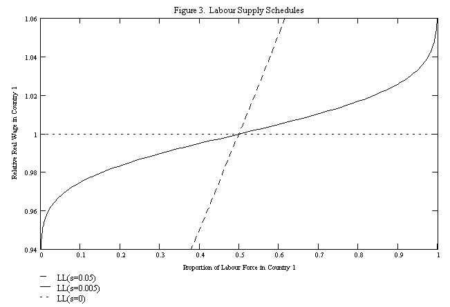
Thus we can calculate the labour supply schedule, showing the relative supply of workers to country 1 given the relative real wage and the degree of disparity in preferences over location. Figure 3 plots various labour-supply schedules. LL(s = 0.05) shows a steep, relatively inelastic schedule, corresponding to a fairly broad distribution of tastes. LL(s = 0.05) plots the a more elastic labour-supply curve where workers need less to induce them to migrate. LL(s = 0) is a perfectly elastic supply schedule corresponding to all workers being indifferent between locations, which is the case implicitly assumed by Krugman (1991a).
Figure 3 here.
4. Equilibrium
We have now established a labour-demand schedule, showing the proportion of the manufacturing labour force that will be employed in country 1 as a function of the relative real wage offered by that country, given the level of international transport costs. We have also found the labour-supply schedule, showing the willingness of workers to take employment in country 1 as a function of the real wage and for particular distributions of preferences over locations in the two-country region. Our next task is to determine the equilibrium employment pattern, resulting from these preferences and transport costs.
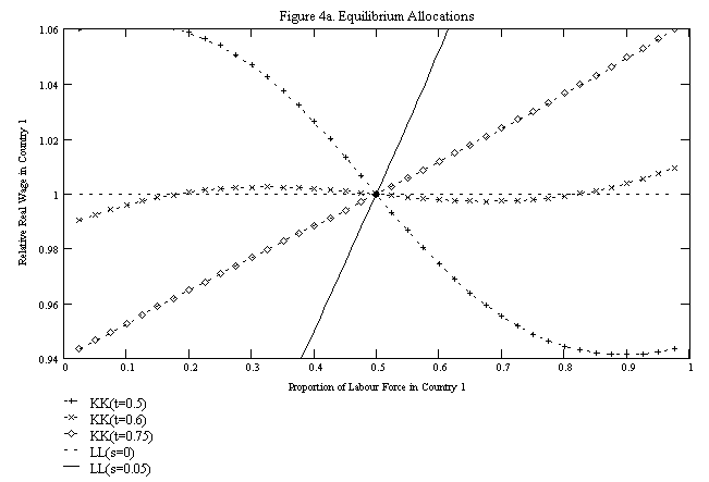
An equilibrium arises either at a point of intersection between the demand and supply schedules (an interior solution) or at either end point, where all of the manufacturing labour is employed in a single country (a corner solution). Not all equilibria are stable solutions: a stable interior equilibrium requires that the labour demand schedule (KK) be flatter than the labour supply schedule (LL) at the point of intersection. A stable corner solution occurs when the LL schedule lies below the KK schedule at f = 0 or when the LL schedule lies above the KK schedule at f = 1 (all manufacturing workers employed in country 2 or country 1, respectively).
Figure 4a here.
If labour is in perfectly elastic supply, as in Krugman (1991a), the labour-supply schedule LL(s = 0), illustrated in Figure 4a, is flat at relative wage w = 1. Three possible configurations of equilibria are possible, depending crucially on the level of the trade costs. The forces of agglomeration are weak when transport costs are high. Thus, when trade costs are high as in KK(t = 0.5), the labour demand curve is downwards sloping, crossing LL(s = 0) from above at the single equilibrium of diversified production, f = 1/2. As trade costs are reduced the labour-demand schedule changes slope as the forces of agglomeration become stronger. At some intermediate levels of trade costs, such as KK(t = 0.6), the labour-demand schedule cuts w = 1 at three points, yielding five equilibria. The interior equilibrium of diversified production (f = 1/2) remains stable and, in addition, the two corner equilibria (corresponding to complete agglomeration in one or other of the countries) are stable, while the other two equilibria are unstable. If transport costs are reduced sufficiently, the labour-demand curve becomes everywhere upwards sloping, as with KK(t = 0.75), and diversification becomes unstable and only agglomerated equilibria are stable.
Now consider the implications of labour being in less-than-perfectly-elastic supply, that is, when the labour-supply schedule slopes upwards. One thing is immediately clear: when the labour-demand schedule is downward sloping, as is the case for KK(t = 0.5) in Figure 4a, a diversified equilibrium will continue to be the only possibility, irrespective of the degree of international labour mobility. However, an inelastic labour supply will mitigate agglomerative forces and diversification may remain a stable equilibrium even when demand linkages are relatively strong. Thus in Figure 4a, the curve LL(s = 0.05) is steeper than KK(t = 0.75) and consequently manufacturing will be spread across the region, despite the agglomerative forces. Agglomeration of manufacturing activity is not an equilibrium in the case of LL(s = 0.05), as this corresponds to a distribution of workers’ preferences over locations such that substantial premia would have to be paid to induce many workers to migrate.
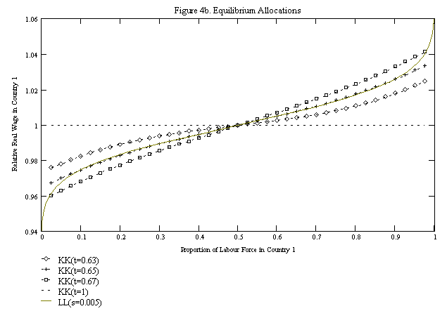
Figure 4b here.
What would be the result were workers, on the whole, less concerned with location? With LL(s = 0.005) workers are closely concentrated around the mean (indifference) and the tails of the distribution are virtually empty. Yet even this degree of locational preference may be sufficient to offset the forces of industrial agglomeration and result in diversification across the region. In Figure 4b, the labour demand schedule KK(t = 0.63) is positively sloped which, if labour were freely mobile, would result in an agglomerated equilibrium. But even with a distribution close to indifference the equilibrium can be diversified production.
However, agglomerative forces may dominate, resulting in agglomeration outcomes becoming stable equilibria in addition to or in place of the diversified equilibrium. Thus KK(t = 0.65) intersects LL(s = 0.005) five times: a stable, diversified equilibrium bounded by two unstable equilibria which are themselves flanked by stable, agglomerated equilibria. But there may now be some workers for whom the economic inducements will never be sufficient for migration. Consequently, the agglomeration is not complete and a small share of the manufacturing labour force remains in the periphery. This is also the case for outcomes where only the agglomerated equilibria are stable, as when the labour-demand schedule KK(t = 0.67) intersects LL(s = 0.005).
This situation is interesting, both in being consistent with casual empiricism (no country is left entirely without a manufacturing sector) and in providing a genuine role for government policy to encourage industrial location (beyond the bang-bang nature of policies when agglomeration is complete and migration incentives lead to a total move of all manufacturing from one country to the other).
How consistent is our model with reality? Let us compare some stylised facts for the US and the EU. The American economy can be characterised as a fully integrated market, with little or no barriers to inter-state factor movements and low internal trade costs. Consequently, it will have an upward-sloping (but not very steep) labour-demand curve and a virtually flat labour-supply schedule. The resulting equilibrium yields a highly agglomerated economy, with a relatively low income differential. In Europe, trade barriers are low, but higher than those in the US, while impediments to factor movements are also greater (for both administrative and cultural reasons). Agglomeration forces may still be strong (KK upwards-sloping), but both the labour-demand and labour-supply curves will be steeper than those of their American counterparts. Manufacturing will have a partially agglomerated equilibrium fairly close to diversification and there will be a higher wage differential than that in the US. Thus the experience of Europe relative to the US is quite consistent with the demand-linkage model.
We have shown that is possible to construct cases where the equilibrium is diversification or partial agglomeration depending on the strength of the agglomerative forces on the labour-demand side and the immobility or unwillingness of labour to move on the supply side. What we now want to show is that, even when labour is initially relatively immobile (as, say, in Europe), the demand-linkages that generate agglomerative forces will be important in determining the response of the region to market integration.
5. Economic Integration
We model economic integration in two ways: the lowering of trade barriers; and an increase in the willingness of labour to migrate. Trade is liberalised as t is increased, free trade being attained when it reaches unity. Improved labour migration will be reflected in weaker locational preferences of all workers (that is, reductions in s), such that a lower premium is necessary to induce each worker to move to the other country.
While liberalisation of trade and factor movements will lead to more efficient production of manufactures within the region, it may have serious distributional consequences. Specifically, whenever agglomeration occurs, those factors left in the periphery will suffer lower real incomes as fewer manufactures are locally produced, resulting in a higher cost of living. The local governments will then have an incentive to try to ensure that the core develops in their country, an issue examined in another paper (Ludema and Wooton, 1997).
With freely internationally mobile labour, trade liberalisation will eventually reach the point at which agglomerative forces are sufficiently strong that the region will jump from having industry dispersed between the countries to a core-periphery pattern of production. Once this jump has occurred, the pattern will be maintained for any further trade liberalisation. This will not, in general, be the outcome of trade liberalisation when labour is less freely mobile between the countries in the region. Instead, two possibilities arise.
Firstly, lowering trade costs will affect the allocation of labour between countries, leading to agglomeration only in situations in which the slope of the labour-demand schedule is positive (so that the forces of agglomeration are strong) and steeper than the labour-supply schedule. Therefore, if the labour-supply line remains steeper than the labour-demand schedule at any level of trade costs, 0 £ t £ 1, then agglomeration will never occur, despite the trade liberalisation. Thus, unless the region has sufficiently mobile workers, agglomerative forces can be held at bay and the region will always have widely dispersed industry. This situation seems to be what Venables (1994) has in mind when he suggests that European migration is "perhaps insufficiently responsive to economic factors" for agglomerative forces "to be of much relevance to European integration."
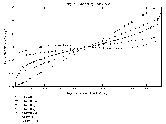
Figure 5 here.
The second, and more intriguing, possibility arises when labour is more freely (but not completely) mobile. This is illustrated in Figure 5 in which LL(s = 0.005) represents a fairly elastic labour supply and the KK schedules show labour demand under increasingly liberal trade (from fairly high trade barriers with KK(t = 0.6) to free trade for KK(t = 1)). In these circumstances demand linkages can certainly have a role to play. The initial stages of trade liberalisation will shift the labour-demand schedule from a negatively sloped function (at the diversified equilibrium of f = 1/2) to one that is positively sloped. As the slope increases, there may be a range of trade costs for which the labour-demand curve becomes steeper than the labour-supply curve at f = 1/2. Consequently, manufacturing will gradually move to a partially agglomerated equilibrium with all but the least mobile workers from one country having moved into the industrial core.
However, this agglomeration will only be a temporary phenomenon as trade liberalisation proceeds. If trade costs continue to fall, the labour-demand schedule gets flatter again, as trade liberalisation weakens the agglomerative forces. (At free trade labour demand is perfectly elastic because, even with demand linkages, there are no benefits to agglomeration if goods can be costlessly moved around the region.) Therefore workers will begin to desert the core and return to their preferred locations. Eventually, trade liberalisation will have progressed sufficiently for the region to return to a stable, diversified equilibrium.
Thus weak locational preferences (less-than-perfectly mobile labour) may result in three phases of trade liberalisation. It may initially drive production from diversification into partial agglomeration and then back into diversification, as the curves cross then re-cross. These effects are qualitatively different from those derived under the assumption of freely mobile labour, both in the temporary nature of the agglomerated equilibrium and the fact that the regional economy does not make discrete jumps between the regimes (of diversification and agglomeration), but gradually adjusts as the intersections between labour-demand and labour-supply curves move to and from geographical concentration of manufacturing.
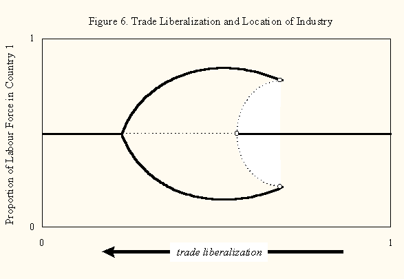
Figure 6 here.
We sketch out the shift from diversification to agglomeration (and back again) as trade is liberalized in Figure 6. Trade liberalization is indicated by declining (1 - t). Stable equilibria are drawn as solid lines, while the dotted lines indicate unstable equilibria. Were labour freely mobile, we would see the now familiar"pitchfork" diagram where trade liberalization initially adds stable agglomerated equilibria to the initial unique equilibrium of diversified production (Venables??, 199?). Further reduction in trade barriers changes the slope of the KK curve and only the diversified equilibria remain stable until all trade impediments are eliminated. Instead of this, we find that the agglomerated equilibria do not involve such an extreme concentration of manufacturing. As trade liberalization progresses, initially the agglomerative forces increase and the equilibria shift further apart. Eventually though, as was pointed out above, continued demolition of trade barriers lessens the incentive for agglomeration. Consequently, the agglomeration will become less pronounced, ultimately disappearing as the region returns to diversified production.
5.2 Increased labour mobility
If economic integration can also take the form of reduced barriers to labour migration (say, in the form of improvements in foreign-language instruction), then the labour-supply schedule will rotate, becoming flatter. When agglomerative forces are weak (the labour-demand schedule being negatively sloped) increased labour mobility, for any given level of trade costs, will have no effect and diversification remains the sole equilibrium.
For stronger demand linkages, the labour-demand schedules will be upward-sloping. If initially the labour supply is relatively inelastic, increased labour mobility may cause the equilibrium allocation to change from diversification to increasing agglomeration as the slope of the labour-supply schedule falls. Thus improving labour mobility will enable agglomerative forces to have increasing effect.
We now consider moves towards establishing a common market in the region with free trade and unrestricted international labour movements. Trade liberalisation is clearly a worthwhile objective in this setting. Indeed, we have shown that completely free trade in goods eliminates the need of movements of factors of production and, consequently, this may be the only policy that the governments of the region need pursue. Though labour mobility would not be necessary to achieve economic efficiency, it may be desirable in meeting the social or political aspirations of the region. The results of the previous two sub-sections indicate that the timing of the two elements of regional integration, trade liberalisation and increased labour mobility, may be crucial in avoiding temporary dislocations in production and local employment.
If labour is initially relatively immobile, trade liberalisation will take place without inducing any international migration. Once a (fairly) liberal trade regime is established, a diversified equilibrium will arise. In that situation factor movements could be allowed, or even encouraged, though no net international movements will be necessary to maintain the diversified equilibrium. If, however, trade liberalisation takes place in the presence of reasonably footloose labour, it might lead to swings towards agglomeration and then back to diversification, with the associated emigrations and return migrations of manufacturing workers. These temporary dislocations in the labour market could cause a great deal of undesirable social upheaval throughout the region.
These problems might be avoided by sequencing the integration policies. Specifically, a restriction on international movements of labour while the trade barriers are being dismantled would suppress the labour migrations that would be induced by the agglomerative forces. These forces decline as trade barriers fall. Hence, once free trade in manufactures has been established, barriers to factor mobility could be reduced.
This policy prescription is already followed by the European Union in agreements with new members. The EU and acceding countries initially eliminate their bilateral tariffs, while restrictions on factor mobility are maintained for several years before being lowered. This ensures that industrial structures can adjust without inducing problems of large, temporary international labour migrations. In particular, it ensures that the acceding country has a better chance of retaining its manufacturing sector and does not experience de-industrialisation through its union with a larger economic entity.
6. Conclusions
This paper uses elements of the new economic geography to examine regional integration. A common market is attained by the elimination of both barriers to trade in goods and impediments to factor mobility. While a lot of attention has been given to the effects of trade liberalisation in models of economic geography, our explicit consideration of issues of factor mobility is both novel and yields outcomes that significantly differ from those where a single regional market for homogenous labour is assumed.
If workers differ in their willingness to move between regions, the equilibrium regional distribution of industry may be affected. Firstly, the reluctance of some workers to move may constrain the forces of industrial agglomeration, leading to countries retaining shares of industrial production which would have been drawn into a core area of the region if labour were more freely mobile. Secondly, even when agglomeration occurs, it will not be complete, as some workers will remain unwilling to migrate in equilibrium.
Trade liberalisation will induce a smoother transition in regional manufacturing activity than occurs with freely mobile labour. However, as a diversified industrial structure will be the equilibrium for both high trade costs and low trade costs, it may be advisable to restrict labour movements until the trade liberalisation phase is complete.
We conclude that economic geography models are indeed relevant to common markets, such as Europe. When demand linkages are sufficient to generate strong agglomerative forces, the national governments will have to take some care in choosing both the depth of integration and the timing of its achievement.
References
Faini, Riccardo (1996), "Increasing Returns, Migrations and Convergence," Journal of Development Economics, 49, 121-36.
Krugman, Paul (1991a), "Increasing Returns and Economic Geography," Journal of Political Economy, 99, June, 483-99.
Krugman, Paul (1991b), Geography and Trade, Cambridge, MA: MIT Press.
Krugman, Paul and A. J. Venables (1995), "Globalization and the Inequality of Nations," Quarterly Journal of Economics, 110, November, 857-80.
Ludema, Rodney D. and Ian Wooton (1997), "Economic Geography and the Fiscal Effects of Regional Integration," mimeo.
Venables, A. J. (1994), "Economic Integration and Industrial Agglomeration," Economic and Social Review, 26, October, 1-17.
Venables?? Reference on pitchfork bifurcations
Notes
Paper presented at a CEPR conference on "Trade and Factor Mobility" held in Venice, 24-25 January 1997. We wish to thank Giorgio Basevi, Julia Darby, Riccardo Faini, and Jim Malley for their help, comments, and suggestions.