March 12, 1998

Department of Economics

Georgetown University

580 Intercultural Center

Washington, DC 20057-1036

Ph: (202) 687-6260

Fx: (202) 687-6102

This paper documents a new "stylized fact" regarding commodity prices using alternative datasets covering the period from 1880 to 1996: The volatility of real commodity prices, defined as nominal commodity prices deflated by the manufacturing unit value index, is higher under flexible-exchange rate regimes than fixed-exchange rate regimes. Furthermore, changes in exchange regime are associated with changes in the persistence of commodity price shocks. Implications of this finding for open-economy macro modeling are briefly discussed in the concluding section.

Key words: Fixed/floating exchange rate regimes; Commodity Prices; Volatility; Time series models

JEL classification: F33; E3; C22

This paper documents a new "stylized fact" regarding commodity prices using alternative datasets covering the period from 1880 to 1996: The volatility of real commodity prices, defined as nominal commodity prices deflated by the manufacturing unit value index, is higher under flexible-exchange rate regimes than fixed-exchange rate regimes. Furthermore, changes in exchange regime are associated with changes in the persistence of commodity price shocks.

Why should we care about this finding? More than40 percent of world trade consists of primary commodities. Both long-term trends and short-term fluctuations in primary commodity prices have important consequences for world economy. On the supply side of the market, many developing countries continue to rely heavily on one or two of these commodities for their export earnings. On the demand side, commodity markets play a non-trivial role in transmitting business cycle disturbances and affecting inflation rates in the industrialized nations (Beckerman and Jenkinson, 1986).

Concerns over possibly adverse long-term trends in commodity prices have occupied development economists at least since the late 1940s. While conclusions regarding long-term trends are mixed, there is general agreement that the volatility of primary commodity export prices is costly for both LDCs and industrial countries. For example, it generates uncertainty in LDC export revenues, which can have negative effects on investment and growth. Moreover, macroeconomic mismanagement in the face of commodity export booms and busts has been a major problem. Understanding the nature of commodity price volatility is a prerequisite for sensible risk management strategies for multinational corporations as well as policymakers.

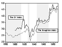
A 1994 World Bank study pointed out that price variability has changed considerably over time, but has been much greater for commodities than for manufacture goods (Figure 1). Reinhart and Wickham (1994), in studying the long-term trend of real commodity prices, find that commodity price volatility is high in the pre-World War II period, subsides in the 1950s and 1960s, rises again in the 1970s, and continues to increase throughout the 1980s and 1990s. Since the 1970s, the volatility of commodity prices has increased almost nine-fold.

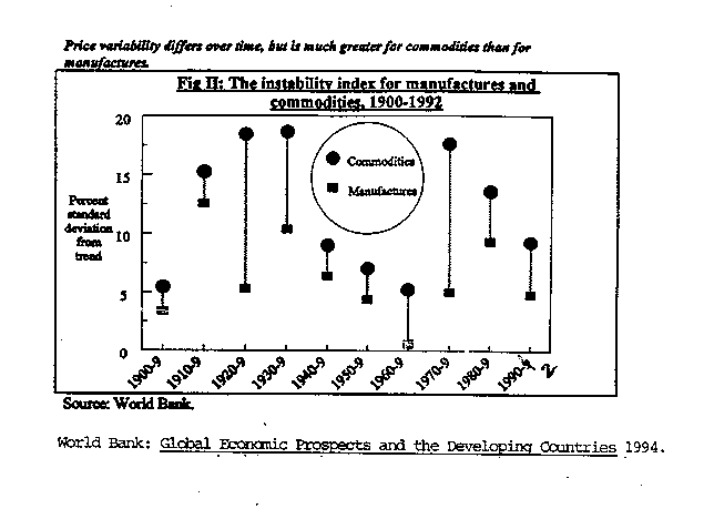Our inspection of Figure 1 raised the question of whether the changes in volatility coincide with changes in exchange rate regimes. Decades when there were flexible exchange rates appear to be accompanied by higher volatility of real commodity prices, but this has yet to be examined in the literature. The purpose of this paper is to carefully examine this hypothesis and briefly discuss its possible implications.

The paper is organized as follows. Section II motivates the study by presenting an overview of commodity price behavior over historical periods characterized by different exchange rate regimes. In order to examine price variability around its long-run trend (or average), the issue of alternative trend specifications is addressed in section III. Section IV discusses the statistical issues involved in identifying volatility changes with regime shifts, and presents the main empirical findings. Section V concludes by discussing the implications of our findings for open-economy modeling of alternative exchange rate regimes.

In this study we consider three alternative data sets collected by (1) Grilli and Yang, (2) Boughton and (3) the IMF, respectively. Following the norm in the commodity price literature, this study examines a real commodity price index, defined as the ratio of the chosen nominal commodity index deflated by the manufacturing unit value (muv) index. The latter is a unit value index for exports from a number of industrial countries.

Grilli and Yang (1988) (GY) constructed a dollar index of 24 internationally traded non-fuel commodity prices from United Nations sources, beginning in 1900 through 1992. They also provide data on an index of muv used as a deflator.

James Boughton (1992) presents a nominal commodity price index and the muv index based on national data and U.N. indexes; it spans the period 1854-1990 and is comprised of 34 non-fuel commodity prices.

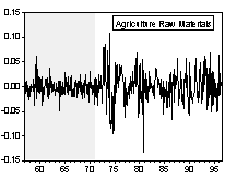
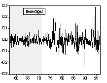
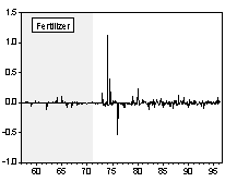
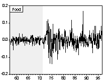
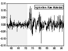
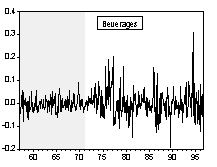
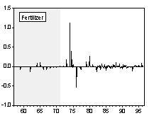
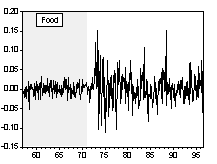
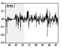
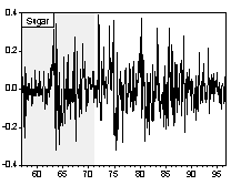
The IMF’s International Financial Statistics (IFS) reports monthly commodity price indexes of agricultural raw materials, beverages, fertilizer, food, metals and sugar from January 1957 through May 1996. These data permit a detailed study of short-run volatility patterns during and after Bretton Woods fixed exchange rate regime.

The post Bretton Woods period has been characterized by a number of major oil shocks, which in turn impacted other commodity prices. Fortunately, the two long-run annual data sets contain exchange rate regime shifts that were not coincident with major oil price shocks. If both long-run and short-run data sets confirm our conjecture, the non-neutrality of exchange regime on real commodity price volatility can be more firmly established.

Before investigating the characteristics of real commodity prices across exchange regimes, this section first provides a brief delineation of the history of the international monetary system by exchange regime.

Over the period for which we have commodity price data, there are three fixed exchange systems. The first is the classical gold standard from 1880 to 1913, a period characterized by fixed nominal exchange rates and essentially no capital controls. The second was the interwar years from 1927 to 1931. Finally, there was the Bretton Woods system from 1946-71. During this period, the dollar was pegged to gold while the other countries pegged to the dollar.

There are three flexible exchange rate episodes during the period studied here. The first episode, which was as close to a free float period as the history records, is between the First World War until the mid-1920s. The second floating exchange episode is 1932-38 when government intervention in the foreign exchange market was pervasive. On August 1971, the devaluation of the dollar brought the Bretton Woods period to a close. Thus, 1972-96 is the final floating rate episode considered.

Using Eichengreen (1994) as a guide, the GY and Boughton data sets are divided into the six subsamples shown in Table 1.

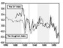
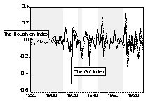
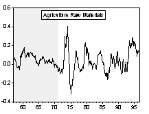
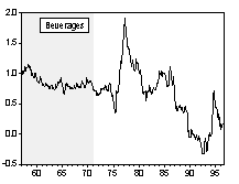
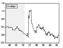
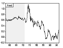
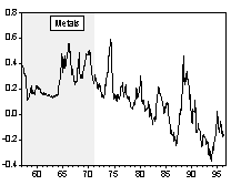
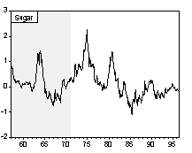
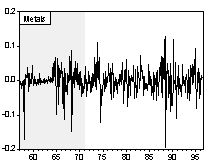
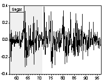
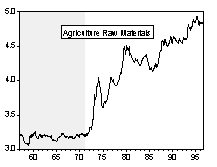
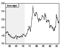
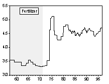
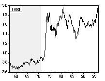
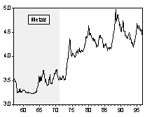
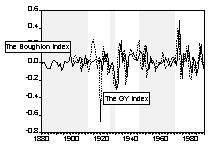
Chart 1 and Chart 2 are graphs of the long-run and short-run real commodity price indices, respectively. Shaded areas correspond to the fixed exchange rate episodes. The evolution of real price indices in log-levels is plotted in part A of the charts, while percentage changes over previous period are shown in part B. (Section III formally examines the series for unit roots.) Simple visual examinations of the data sets point to striking differences in the real commodity price behavior across exchange rate regimes. It appears that prices were relatively tranquil during the fixed exchange episodes and became much more volatile during the flexible exchange periods. A simple statistical summary is presented in Table 2.

Before investigating the volatility behavior across different exchange regimes, we first test the simple hypothesis that the volatility is constant across the various fixed (flexible) rate periods for the long-run data sets. Suppose that D log(y_t) (y_t being the real commodity price) is normally distributed, we can then use analysis of variance (or ANOVA) method to test the null hypothesis of equal variance across the various fixed (flexible) exchange rate episodes. The results indicate that the null can not be rejected for either fixed or flexible exchange regimes. The test statistics along with the critical values are reported in Table 3.

Given that we failed to reject the hypothesis that the commodity price variance is equal across the various fixed (flexible) exchange rate periods, we can then proceed to test whether the variance is equal across the two regimes. The test results reveal clear rejection of the null of equal variance: The F statistics are 2.62 for the GY and 4.02 for the Boughton data set, with the critical value of rejecting the null being 2.11 and 2.02, respectively. However, because of the violation of the normality assumption in D log(y_t), the exact confidence levels of the test should not be taken too literally. A more systematic study of this issue is presented in section IV.

Before measuring the temporal variation in the second moments of a time series, it is important to consider alternative specifications of its trend. One disagreement among scholars testing the PS hypothesis has been whether the difference stationary (DS) or the trend stationary (TS) model should be employed to describe the underlying data generating process.

In light of these mixed results, this study will first analyze the three data sets by testing for the presence of unit roots. The model is specified as follows.

(1)

(2)

where log y_t is the natural logarithm of real commodity price index. The error process in (2) has been written with the largest root factored out. It is assumed that the lag polynomial A(L) is invertible and B(L), hence A(L)^-1B(L), are stable polynomial lag operators. e _t is serially uncorrelated with zero mean and finite variance.

If r =1 in equation (2), the error process is said to have a unit root. In this case, the correct procedure is to first difference equation (1). However, if there is no unit root in equation (2), first difference the model will introduce a unit root into the MA part of the error process. The presence of unit root is investigated using the Phillips-Perron test, which examines the statistical significance of r in the following regression equation:

(3)

where f =r -1 and dlogy_t represents the first difference of the logarithm of the underlying data.

The equation is estimated by ordinary least squares and then the t-statistic for the null hypothesis f = 0 (or equivalently r =1) is corrected for both heteroskedasticity and autocorrelation using Newey-West (1987) procedure. The appropriate distribution of the test statistics depends on whether the constant term and time are included in (3). Equation (3) is first estimated with both a constant and a time trend included. If the null hypothesis that there exists a unit root (i.e., f = 0) is not rejected for the least restrictive specification, the significance of the trend and constant terms are examined in turn to see whether the test can gain more power by dropping one or both terms. If the null is rejected at any stage, we proceed no further (Enders, 1995).

Table 4 reports the results of the Phillips-Perron tests on the GY, the Boughton and the IFS data sets. For the real price series, the null of f = 0 is rejected at the 5% significance level for the monthly series of agricultural raw materials, metals and sugar. The third column indicates whether a time trend (T), or a constant (C), or neither term (N) is included in the variant of equation (3) that was chosen using the method described in the previous paragraph.

The long-run time series data permit the investigation of commodity price volatility across three fixed and three flexible exchange regimes. The empirical strategy used here to test for volatility shifts across exchange regimes is to use dummy variables in the residual series: that is, the error variance in (2) takes the form:

DumFLEXIBLE is the dummy variable that takes the value 0 for fixed exchange period and 1 for flexible exchange period. We can then test whether flexible exchange regime has been associated with a statistically different variance than the fixed exchange regimes. The regime shift dates are those shown in Table1.

Since previous studies using the GY and the Boughton data sets have reported mixed results on the unit root test, we consider both TS and DS specifications. It can then be seen whether any test results on volatility shifts are sensitive to the detrending method employed.

First, the autocorrelations and partial autocorrelations (ACFs and PACFs) of the squared residuals from either the TS or the DS model are examined to determine the appropriate length in A(L) and B(L). Diagnostic checks are done using correlograms and Ljung-Box Q-statistic to make sure that there is no further serial correlation in the residuals. The hypothesis that the variances of e _t are the same across different exchange regimes amounts to testing H_o: m ₂=0 in model defined by (1), (2) and (4).

The test results are summarized in Table 5. The Newey-West Heteroskedasticity consistent covariance is used and the t-statistics are in parentheses. It can be seen that, regardless whether the TS or DS model is specified, m ₂ is significantly different from zero at the 5% level. Volatility of real commodity price differs across exchange regime. Furthermore, the magnitude of m ₂ measures how much the volatility associated with the flexible exchange regimes differs from that of fixed exchange regimes. Since m ₂ is significantly positive in every specification considered, there is strong evidence that flexible exchange rate regimes have been associated with a much higher real commodity price volatility than fixed exchange regimes.

Table 5. Estimated values of m ₂ and relevant t-statistics

The last section presented some strong evidence of volatility shifts across exchange regimes using annual data series. However, the limited number of observations during some of the brief exchange regime episodes may leave skeptical readers unconvinced. Hence, in this section the IMF’s monthly commodity price series are investigated to see whether there is a change in variance associated with the breakdown of Bretton Woods fixed regime. We use a univariate generalized autoregressive conditional heteroskedastic model (GARCH) to account for time varying variances and covariances. The hypothesis is to examine the extent to which the change in nominal exchange regime leads to parameter shifts in the GARCH process for commodity prices. If GARCH parameters vary with exchange regime shifts, this implies changes in the degree to which shocks to commodity price volatility persist over time.

The first part of the exercise is to examine whether GARCH provides a good description of the behavior of the six monthly commodity price series, ignoring the possible regime shift effects on the conditional variances. Exchange rate regime shifts are then introduced

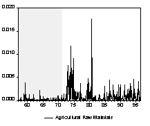
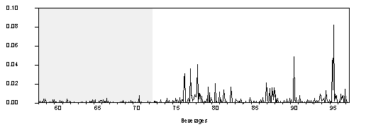
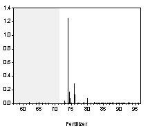
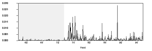
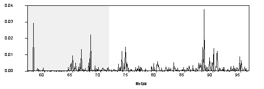
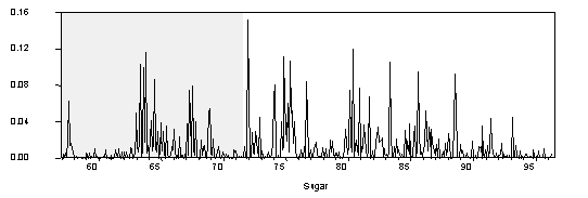
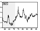
It has long been observed that asset returns tend to be leptokurtic (i.e. they exhibit "fat tails"). In many ways, commodity prices behave like asset prices. Not surprisingly, visual inspections of the commodity price series reveal volatility clustering. Large changes tend to be followed by large changes, and small changes tend to be followed by small changes (see Chart 3).

Engle’s (1982) autoregressive conditional heteroskedastic (ARCH) model allows for persistence in conditional variance by specifying an autoregressive structure on the squared residuals. After an appropriate specification of the conditional mean using equations (1) and (2), the residual e _t is modeled as an ARCH(m) process.

(5)

(6)

where I_t-1 is the information set through time t-1.

e _t is serially uncorrelated but not stochastically independent because they are related through their second moments. In order for e _t² to be positive and covariance stationary, the following restrictions are required on the coefficients in equation (5): a ₁>0, _{a i³} 0 for i=1,2,...,m, and a ₁+a ₂+...+a _m<1. In practice, arbitrary declining weight structures are usually imposed to meet these coefficient restrictions.

Bollerslev (1986) develops the GARCH model which extends the ARCH(m) model to allow the conditional variance to be an ARMA process. Hence, instead of equation (6), the conditional variance is specified as:

(6’)

The variance today depends on past news about volatility (the e _t² terms) and past forecast variance (the h_t terms). The inclusion of lagged conditional variances might capture some sort of adaptive learning mechanism. The benefit of the GARCH specification (6’) is that it is more parsimonious and entails fewer coefficient restrictions than equation (6). Sufficient conditions for well-defined variance and covariance only require all coefficients in equation (6’) to lie inside the unit circle. For example, in a GARCH(1,1) process, it requires a >0, b >0, and a +b <1.

For asset prices, it is often observed that downward price changes are followed by higher volatilities than upward movements of the same magnitude. Glosten, Jagnanathan, and Runkle (1989) proposed the Threshold ARCH (TARCH) specification to model the conditional variance as:

(6’’)

where d_t =1/2 if e _t<0 and 0 otherwise. Hence, positive e _t has an impact of a (L) on the conditional variance while bad news has an impact of a (L)+g (L).

For most financial time series, GARCH(1,1) provides a sufficiently good fit. This is also true for the monthly commodity price series, except in the case of fertilizer. For real metal price series, TARCH(1,1) provides a better fit. The TARCH term is negative, implying that upward price spikes increases volatility. All ARCH and GARCH terms are significantly greater than zero. The strength of this significance is one indication of the appropriateness of the GARCH specification for the commodity price data.

Table 6. Estimation of the GARCH(1,1) model (1951 January—1996 May)

Table 6 presents the test statistics for both the mean and variance estimation, using the appropriate trend models according to the unit root test results in Table 4. Diagnostic checks (correlograms and ARCH LM tests) confirm that there is no further serial correlation, nor ARCH effects, in the residuals.

The squared residual can be decomposed into its conditional expectation (h_t) plus an innovation (v_t) term. The latter by definition is unpredictable based on the past:

(7)

Substituting equation (7) into (6’), an alternative expression for the squared residuals is as follows:

(8)

It can be seen that the squared errors follow an ARMA(1,1) process, although v_t is not a white noise innovation. While the conditional variance of e _t is E_{t-1e t}²=h_t, the unconditional variance exists when a +b +g /2<1. It is defined as:

(9)

When s ² exist and is independent of time, the GARCH process is stationary. The sum of a , g /2 and b measures the persistence of volatility shocks. For many commodity series, this sum is very close to unity and shocks die out rather slowly. For real food price indices, the sum is greater than one. When a +b +g /2=1, the ARMA process for e _t² would have a unit root and the GARCH process is said to be integrated in variance (IGARCH) (Engle and Bollerslev, 1986). In this case the unconditional variance of e _t is infinite, even though it is still possible for e _t itself to be a strictly stationary process (Nelson, 1990). For IGARCH process, "current information remains important for the forecasts of the conditional variances for all horizons" (Engle and Bollerslev, 1986, p27).

The purpose of this subsection is to test whether s ² in (9) is constant over time or it depends on the shifts in the exchange rate regimes.

It is potentially restrictive to assume that d is constant over time, especially given the nature of the world economy during the sample period. Shifts in exchange regimes, which may lead to shifts in policy parameters of national governments and/or shifts in the optimal response functions of market participants, may cause changes in the conditional and unconditional variances, implying a nonstationary GARCH process.

To examine this contention empirically, a dummy variable, FLEXIBLE, indicating the presence of a flexible exchange regime, is used in the conditional variance equation. The likelihood ratio tests can be used to test parameter shifts in the commodity price process by nesting the restricted process within a general unrestricted process:

where FLEXIBLE=1 for observations in subsample starting from August 1971 and 0 otherwise. Equation (10) reduces to equation (6) when d ₂=0 (i.e., d ₁=d ), that is, when the intercept is independent of the exchange regimes.

The estimation results in Table 7 show that d ₂ is statistically different from zero for all series except the real fertilizer price index. In addition, including the regime shift dummy significantly improves the fit of the model. The likelihood ratio statistic, which tests the restriction of d ₂=0, is significant at less than 5% level in all cases. Furthermore, the flexible exchange regimes is associated with a much higher conditional variance and hence a higher unconditional variance.

In addition, the sum of a and g /2 plus b clearly declines in all cases when regime shift is accounted for. Diebold (1986, p.55) suggests that regime shifts may cause the appearance of integrated ARCH. The evidence reported here supports his conjecture. For real food price series, this sum is no longer more than one. Hence, if there are regime shifts in the underlying data generating process, failing to account for it may lead to conclusions that shocks to volatility are more persistent than they actually are.

Table 7. Accounting for Exchange Regime Shift in the GARCH(1,1) model

This paper investigates differences in real primary commodity price volatility across fixed and flexible exchange rate regimes. The findings suggest that exchange arrangement may imply an important source of systematic risk to world commodity trade. Using three different data sets over different sample periods, as well as alternative detrending methods, there is strong evidence supporting the conjecture that the flexible exchange periods have been associated with a higher real commodity price volatility than the fixed exchange periods. Also, regime shifts play a nontrivial role in determining volatility persistence.

These conclusions regarding commodity price volatility should be of interest to international macroeconomists, not just those studying global commodity markets, for several reasons. The puzzle of why commodity price volatility varies with exchange rate arrangement may well be related to a puzzle in the literature regarding fundamental determinants of the exchange rate. Flood and Rose (1995) show that there are no significant changes in the time series processes of output, money, nor prices across exchange regimes. Since the volatilities of nominal exchange rates exhibit apparent shifts across exchange regimes, they conclude that the above macro aggregates can not be the true fundamentals for exchange rates. It would be interesting to see whether this problem of identifying underlying fundamentals is also present in international commodity markets.

Empirical studies of business cycles in open economies have sometimes concluded that the nominal and real exchange rates are virtually the only macroeconomic variables that have experienced dramatic changes in volatility across exchange rate regimes. Interestingly, Grilli and Kaminsky (1991) have recently argued that even real exchange rate behavior is regime-independent if one considers a broader historical perspective using monthly data from 1886 to 1986. Their results, however, are very sensitive to whether particular subperiods are included in the analysis. In any event, using roughly the same one hundred year period, our results show quite unambiguously that the relative prices of primary commodities in terms of manufactures have time series characteristics that vary across exchange rate regimes.

From a theoretical standpoint, our findings have implications for the plausibility of various macroeconomic models used in studying alternative exchange rate regimes. As Stockman (1983) highlights, two types of models have been used in the literature on real exchange rate volatility across regime. Sticky-price models (e.g., Dornbusch (1976), Frenkel (1981), and Mussa (1982)) exhibit nonneutrality with respect to the nominal exchange rate regime. Adopting floating exchange rates implies higher nominal and real exchange rate variability. In contrast, a class of equilibrium models (see, e.g., Helpman (1981), Lucas (1982) and Stockman (1980)) satisfies "the nominal exchange regime neutrality proposition," i.e. the time series properties of all real variables are invariant to the choice of exchange regime. Hence, the alleged difference in real exchange rate behavior across exchange regimes has generally been viewed as a consequence of price stickiness. Stockman illustrates, however, that some equilibrium models, for example those with nontradeable as well as tradeable goods – not just sticky price models – may also exhibit nonneutrailities with respect to the exchange rate regime.

Our analysis focuses on two types of internationally traded goods; primary commodities and manufactures. It remains to be determined whether our finding that the relative price of these two tradeable goods increases under flexible exchange rates can be explained in the context of equilibrium models, even those described by Stockman as exhibiting nominal exchange rate nonneutrality. This is a topic of our ongoing research. The empirical results here suggest that the mechanism linking the exchange rate with primary commodities may be different from that of manufactured goods. This in turn seems to reflect some form of price stickiness, perhaps arising from different market structures for the two types of goods. Recent work by Goldberg and Knetter’s (1997) also concludes that empirical price-exchange rate relationship may reflect underlying differences in market structure across industries.

This appendix summarizes our analyses of nominal commodity price volatility. The results are qualitatively similar to those obtained in the text using real price indices.

Simple visual examinations of Chart 1 and 2 point to striking differences in the nominal commodity price behaviors across exchange rate regimes.

Most nominal price indices are found to have a stochastic trend. The Phillips-Perron tests on unit root show that the null hypothesis of r =1 can not be rejected at the 5% significance levels, except for the series of sugar prices.

For the two long-run nominal commodity price series, the null hypothesis that volatility does not change significantly across exchange regimes can be rejected at the 5% level, regardless of which trend specification is used. The test results are summarized in Table 3.

For the monthly price series except fertilizer, the GARCH (1,1) model provides a sufficiently good fit. For the price series of agricultural raw materials, TARCH(1,1) provides a better fit. The test statistics for both the mean and variance estimation are presented in Table 4. The sum of a , g /2and b measures the persistence of volatility shocks. For the series of food and metals, the sum is more than one.

Accounting for the regime shift in the GARCH process significantly improves the fit of the model. In addition, the degree of shock persistency clearly declines. Recall that Diebold (1986, p.55) suggests that regime shifts may cause the appearance of integrated ARCH. The evidence reported here supports his conjecture: The sum of a , g /2 plus b is no longer greater than one except for the nominal price of metals once regime shifts are allowed.

This appendix summarizes our analysis of the long-run data series when structural break in 1920 is allowed in the specification of equation (1):

(1’)

where Dum1920 is the dummy variable that takes the value 1 for data in 1920 and 0 otherwise. The test results of equation (4) are presented in the following table. It can be seen that, regardless whether the structural break is allowed or not (in either the TS or the DS model), m ₂ is significantly different from zero at the 5% level. Hence, it further confirms our conjecture that volatility of real commodity price differs across exchange regime.

References

Baxter, M and A.C. Stockman. 1989. "Business Cycles and the Exchange-Rate Regime: Some International Evidence," Journal of Monetary Economics 23, 377-400.
Beckerman, W. and T. Jenkinson. 1986. "What Stopped the Inflation? Unemployment or Commodity Prices?" Economic Journal 96, 39-54.
Bollerslev, T. 1986. "Generalized Autoregressive Conditional Heteroscedasticity," Journal of Econometrics 31, 307-27.
Bordo, M.D. and A.J. Schwartz. 1996. "Why Clashes between Internal and External Stability Goals End in Currency Crises, 1797-1994," Open Economies Review 7, 437-68.
Boughton, J.M. 1991. "Commodity and Manufactures Prices in the Long Run," International Monetary Fund Working Paper, WP/91/47.
Cuddington, J.T. 1992 "Long-Run Trends in 26 Primary Commodity Prices: A Disaggregated Look at the Prebisch-Singer Hypothesis," Journal of Development Economics 39. 207-227.
Cuddington, J.T. and C.M. Urzúa. 1989. "Trend and Cycles in the Net Barter Terms of Trade: A New Approach," Economic Journal 99, 426-442.
Deaton, A and G. Laroque. 1992. "On the Behaviour of Commodity Prices," Review of Economic Studies 59, 1-23.
Diebold, F.X. 1986. "Modeling Persistence in Conditional Variances: A Comment," Econometric Reviews 5, 51-56.
Dornbusch, R. 1976. "Expectations and Exchange Rate Dynamics," Journal of Political Economy, 84, 1161-1176.
Eichengreen, B. 1994. "History of the International Monetary System: Implications for Research in International Macroeconomics and Finance," Chapter 6 in F. Ploeg ed. Handbook of International Macroeconomics, Blackwell, Oxford UK & Cambridge USA. 153-197.
Enders, W. 1995. Applied Econometric Time Series, John Wiley & Sons, Inc.
Engle, R.R. 1982. "Autoregressive Conditional Heteroskedasticity with Estimates of the Variance of United Kingdom Inflation," Econometrica 50, July, 987-1007.
Engle, R.F. and T. Bollerslev. 1986. "Modeling the Persistence of Conditional Variances," Econometric Reviews 5, 1-50.
Flood, R.R. and A.K. Rose. 1995. "Exchange Rates: A Virtual Quest for Fundamentals," Journal of Monetary Economics 36, 3-37.
Frenkel, J. 1981. "Flexible Exchange Rates, Prices and Role of "News": Lessons from the 1970s," Journal of Political Economy, 89, 665-690.
Glosten, L.R.. R. Jagannathan and D. Runkle. 1989. "Relationship between the Expected Value and the Volatility of the Nominal Excess Return on Stocks," Northwestern University. mimeo.
Goldberg, P.K. and M.M. Knetter. 1997. "Goods Prices and Exchange Rates: What Have We Learned?" Journal of Economic Literature XXXV, 1243-1272.
Grilli, V. and G. Kaminsky. 1991 "Nominal Exchange Rate Regimes and the Real Exchange Rate: Evidence From the United States and Britain, 1885-1986," Journal of Monetary Economics 27, 191-212
Grilli, E.R. and M.C. Yang. 1988. "Primary Commodity Prices, Manufactured Goods Prices, and Terms of Trade of Developing Countries: What the Long Run Shows," World Bank Economic Review 2(1), 1-48.
Helpman, E.1981. "An Exploration in the Theory of Exchange-Rate Regimes," Journal of Political Economy, 89, 865-890.
Lastrapes, W.D. 1989. "Exchange Rate Volatility and U.S. Monetary Policy: An ARCH Application," Journal of Money, Credit and Banking 21(1), 66-77.
Lucas, R. 1982. "Interest Rates and Currency Prices in a Two-Country World," Journal of Monetary Economics, 10, 335-360.
MacKinnon, 1991. "Critical Values for Cointegration Tests," in Engle and Granger eds., Long-Run Economic Relationships: Readings in Cointegration. Advanced Texts in Econometrics. Oxford, New York, Toronto and Melbourne: Oxford University Press. 267-76.
Mussa, M. 1982. "A Model of Exchange Rate Dynamics," Journal of Political Economy, 90, 74-104.
Mussa, M. 1986. "Nominal Exchange Rage Regimes and the Behavior of Real Exchange Rates: Evidence and Implications," in Carnegie-Rochester Conference Series on Public Policy 25, 117-214.
Nelson, D.B. 1990. "Stationarity and Persistence in the GARCH(1,1) Model," Econometric Theory 6, 318-34.
Newey, W.K. and K.D. West. 1987. "A Simple Positive Semi-Definite, Heteroskedasticity and Autocorrelation Consistent Covariance Matrix," Econometirca 55, 703-8.
Perron, P. 1990. "Testing for a Unit Root in a Time Series with a Changing Mean," Journal of Business and Economic Statistics 8, 153-162.
Powell, A. 1991. "Commodity and Developing Country Terms of Trade: What Does the Long Run Show?" Economic Journal 101, 1485-96.
Prebisch, R. 1950. The Economic Development of Latin America and its Principal Problems. United Nations, Lake Success.
Reinhart, C.M and P. Wickham. 1994. "Commodity Prices: Cyclical Weakness or Secular Decline?" International Monetary Fund Staff Papers 41(2), 175-213.
Rogers, J.H. 1995. "Real Shocks and Real Exchange Rates in Really Long-Term Data," International Finance Discussion Papers, Board of Governors of the Federal Reserve System. No. 493.
Singer, H. 1950. "The Distributions of Gains between Investing and Borrowing Countries," American Economic Review, Papers and Proceedings May, 473-485.
Stockman, A. 1980. "A Theory of Exchange Rate Determination," Journal of Political Economy, 88, 673-698.
Stockman, A. 1983. "Real Exchange Rates under Alternative Nominal Exchange-Rate Systems," Journal of International Money and Finance, 2, 147-166.
World Bank, 1994. Global Economic Prospects and the Developing Countries. Washington, DC.
Appendix 1: Analysis of Nominal Commodity Price Volatility