A New Bayesian Model of Market Microstructure Behaviour Applied to the Market in Irish Government Securities; Identification Happens!
By
Peter G. Dunne
The Queen’s University of Belfast
Sept. 1998
ABSTRACT:
For the case of a market-making trading environment, this study shows how a vector moving average representation of transaction price returns and trade can be decomposed to a finer degree than before so as to reveal, not just summary measures of Microstructure characteristics, but also estimates of the components that make up these measures. This additional information reveals the source of differences in microstructures rather than merely measuring the effects of these differences. Quite a general theoretical model underpins the empirical application and this provides a framework for the analysis of trading cost components and the information content of trade. The new approach is applied to the case of the Irish market in government securities.
I. INTRODUCTION:
The analysis of financial market microstructure is now a well established topic in the field of applied information economics. All kinds of financial markets have been analysed using the tools developed in this field, (although seldom the markets in government securities). The topics chosen for most attention within this category is the measurement and comparison of trading costs across markets, represented by components due to order processing costs and costs due to asymmetric information and inventory control mechanisms. Some good examples of the empirical microstructure literature in this vein include, Garman (1976), Roll (1984), Copeland and Galai (1983), Glosten (1987), Glosten and Milgrom (1985), Glosten and Harris (1988), Harris (1990), Choi, Salandro and Shastri (1988), Stoll (1989), George, Kaul and Nimalendran (1991), Hasbrouck (1991a, 1991b, 1993, 1998), Hasbrouck and Ho (1987), Hasbrouck and Sofianos (1993), Madhavan and Smidt (1991, 1993) and Snell and Tonks (1996, 1997). The more theoretical microstructure literature has been surveyed by O’Hara(1995).
Although the empirical microstructure literature has made extensive use of the existing tools of time-series econometrics, and despite the increasing quantity and quality of the data analysed, there are still a number of microstructure variables that defy accurate identification and measurement. For example, the measure of market quality proposed by Hasbrouck (1991), (applied in the context of Gilt markets by Dunne, 1994 and Proudman, 1997), uses a vector autoregression of high frequency returns and trades, and provides a measure of market quality, which can only be regarded as an approximate lower-bound estimate, of the size of trading costs. Another example of incomplete identification or inaccurate measurement, is the Bayesian approach taken by Madhavan and Smidt(1991), in which it is assumed that agents arrive in each transaction period with no prior belief about the value of the asset being traded.. Despite this unappealing assumption, and other deficiencies discussed below, this model stands as one of the more acceptable measures of this important microstructure variable. While others, such as Snell and Tonks(1996), have proposed alternatives to the Madhavan and Smidt application, these alternatives tend to rely on other equally unappealing restrictions. For example, Snell and Tonks do not use a Bayesian framework and they assume that separate news shocks arrive in each transaction period and that the private news shock is observed without noise. The private information is therefore the source of a pure speculative opportunity without risk. As is well known in the microstructure literature, the measurement of order processing and inventory control costs is highly sensitive to the correct measurement of the asymmetric information component of trading costs, and for this reason, it is difficult to conclude at this point that we possess empirical methods that provide reliable measures of any of the main trading cost components.
In this study, the more realistic and useful aspects of at least two of the main contributions mentioned above are combined to give rise to an empirical application which does not suffer from the more obvious weaknesses of any one of these contributions taken individually. The model which is selected as the corner stone and basis for generalisation and improvement is that of Madhavan and Smidt (1991). The empirical approach adopted is along the lines of the Hasbrouck (1993) approach to the measurement of market quality. While there are a number of problems with the Madhavan and Smidt application, the behavioural model upon which it is based has good properties. The original application by Madhavan and Smidt resulted in a single equation econometric model, but it is shown below that, with very little modification, the same model can be represented as a two equation vector moving average representation (VMA) involving transaction price returns and trade-quantity. The benefits accruing to the use of transaction price returns rather than quote data have been documented elsewhere and relate to the fact that a significant proportion of trades take place within the best market spread, (e.g., Naik and Yadav, 1997). In any case, the quote data was not available for use in the application below.
As is well known from the time series literature, e.g., Beveridge and Nelson(1981) and Watson(1986), VMA representations can be decomposed into trend and stationary components. Furthermore, it is often possible to impose theoretically motivated restrictions on the estimation results from, what is sometimes referred to as, the ‘standard-form’ of these representations, in such a way as to provide identification of the underlying primitive innovations of a theoretical model. The best known example is that due to Blanchard and Quah (1989), where the residuals from a standard-form VAR in GNP and unemployment is decomposed into demand and supply shocks. An approach which relates theoretical and empirical models in this way has not yet been applied in the microstructure field. While Hasbrouck’s measure of market quality is based upon the stationary innovation variance in the transaction price series this measure was only loosely related to a theoretical model of behaviour. The analysis below brings this general approach a significant step forward by grounding the decomposition of transaction prices and trades in a Bayesian model of behaviour in such a way that the empirical application identifies the important microstructural parameters.
Thus, it is shown below that the decomposition strategy can be used in the case of VMA representation of a revised Madhavan and Smidt model of microstructural behaviour. The restrictions derived from the theoretical model are related to the discipline imposed by Bayesian rules for up-dating conditional expectations. These restrictions allow for a complete identification of the various components of microstructure parameters previously measured in the literature. Furthermore, the approach gives a complete breakdown of the parameters which describes the average weight placed on the information signals received by both the market maker and informed traders. The measures which result are much more informative than those already in existence. It is possible to identify the components of the existing measures so that the causes of differential market quality can be determined. This additional information would help to identify those markets in which private information is more valuable and those situations in which informed trades can best be disguised. These factors are interesting because they relate directly to the whole issue of market liquidity and depth.
The approach developed here is applied to Irish market in Government Securities which changed from an agent-only system of trading to a market-making system in late 1995. It has been suggested in some quarters of the microstructure literature, most notably Proudman(1995), that the gilt market is not characterised by information asymmetry. Proudman provides some evidence to this effect but has used one of the techniques suffering from the deficiencies already mentioned above. The classic form of information asymmetry occurs in equity markets and is often associated with "insider trading". While it is true that gilt markets are not likely to suffer from such severe asymmetries, it can also be argued that these markets may involve influential traders who could be instrumental in guiding market opinion by their trading behaviour. It is possible that these influential opinion leaders are also the largest speculators and that their trades contain information about the likely future path of the overall market’s valuation of a stock. The results obtained below, in fact, provide supporting evidence to that of Proudman, and indicate that there is an insignificant information content of trade in the Gilt-edged securities markets. It appears that the only source of risk for the market maker is that related to inventory control. This evidence is useful in settling the issue about influential traders and it is also useful in providing a test run of the new empirical approach.
In conclusion, the steps taken to arrive at the new empirical measures of market microstructure can be described as; (i) generalise and improve upon the Bayesian model of microstructure behaviour proposed by Madhavan and Smidt (1993), (ii) state the theoretical model as a VMA in terms of the underlying transitory and permanent innovations; call this the ‘primitive-form’ and take note of any restrictions implied by the theoretical model which may impinge upon estimation of a possible empirical model, (iii) estimate an appropriate corresponding empirical model taking into account any restrictions implied by the theoretical model and call this the ‘standard-form’ result, (iv) use the variance-covariance matrix of the standard-form transitory innovations along with the corresponding variance-covariance matrix implied by the theoretical model to identify the microstructure parameters of interest.
The remainder of this paper is arranged as follows. Section II considers the Bayesian model of Madhavan and Smidt and introduces an alternative model which has more appealing properties. This section also discusses the deficiencies associated with the single equation empirical approach taken by Madhaven and Smidt. Section III considers how the theoretical model can be stated in vector form and how the theoretical model relates to a corresponding ‘standard-form’. It is then shown how the correspondence between these representations gives rise to identification of various microstructural parameters. Section IV discusses the special features of the data and describes how the Kalman filter is used to achieve estimates of the parameters of interest. Section V contains an interpretation and discussion of the results from an application of the new technique. Section VI contains a summary and conclusion.
There are a number of possible assumptions that could be made regarding the formation of beliefs on the part of information processors in the analysis to follow. The first case to consider is that used by Madhavan and Smidt. The Madhavan and Smidt model is considered to be too restrictive to be of any use in the current analysis. In that model the authors assumed that the past value of the asset being traded has no contribution to make towards the current formation of beliefs about current underlying value. In other words, they assume that on arrival into a new transaction period all agents are asked to forget all past information shocks and to use the current public information shock as their prior belief about the ‘true’ vale of the asset being traded. An alternative model assumes a common prior equal to the previous period’s value. This assumption is a vast improvement over the Madhavan and Smidt case and might appeal to those who believe that private information is short lived. Indeed, it might be a good description of the case in which all market makers are required to reveal the size of their most recent trades.
There are three type of agents interacting in this model namely, the market maker, informed traders and noise traders. The behavioural model begins with the assumption that in each transaction period a public trader asks the market maker for his quote, (or schedule of quotes for different sizes of trade), and given this quote he decides whether and how much to trade. This differs from the market making situation in which quotes are electronically posted. Snell and Tonks (1997) make use of this difference in their analysis of quote data from the London Stock Exchange but it is easy to show that this is not an issue of consequence when dealing with transactions data. The transaction-to-transaction price change will reflect both the public information innovations and the information content of trade and the cleaving of the price change into its components is what provides the main difficulty for the econometric modeller.
The underlying value of the asset at time t, (or the implicit efficient price), is denoted ![]() 1. This will be the permanent component of price movements and it follows a random walk with zero mean iid normal increments denoted
1. This will be the permanent component of price movements and it follows a random walk with zero mean iid normal increments denoted ![]() with variance
with variance ![]() . The transaction price,
. The transaction price, ![]() , that is observed in period ‘t’ is equal to the quote relevant for the type of trade that occurs at time ‘t’. It is assumed that the market maker sets quotes that, (in addition to reflecting inventory and order processing costs), will be ‘regret-free’ in the sense of Glosten and Milgrom (1985).2 In this way the quote that becomes the transaction price already embodies the information in the trade. Price can therefore be described by;
, that is observed in period ‘t’ is equal to the quote relevant for the type of trade that occurs at time ‘t’. It is assumed that the market maker sets quotes that, (in addition to reflecting inventory and order processing costs), will be ‘regret-free’ in the sense of Glosten and Milgrom (1985).2 In this way the quote that becomes the transaction price already embodies the information in the trade. Price can therefore be described by;
![]() (1)3
(1)3
where;
![]() 4is the expectation of
4is the expectation of![]() 5conditional upon the market maker’s information at time t,
5conditional upon the market maker’s information at time t, ![]() 6is the level of inventory at time t, (this can be replaced by the term
6is the level of inventory at time t, (this can be replaced by the term ![]() where
where ![]() is non-zero level of desired inventory),
is non-zero level of desired inventory),![]() 7is an indicator +1 for a buy and -1 for a sell, and
7is an indicator +1 for a buy and -1 for a sell, and![]() and
and ![]() are constant coefficients.
are constant coefficients.
The order quantity ![]() 8 obeys the following relation;
8 obeys the following relation;
![]() (2)9
(2)9
where;
![]() 10is some positive constant,
10is some positive constant, ![]() 11is the informed trader's conditional expectation of
11is the informed trader's conditional expectation of![]() 12given his information at time t, and
12given his information at time t, and ![]() 13 is an idiosyncratic iid normal innovation with variance
13 is an idiosyncratic iid normal innovation with variance ![]() , that represents liquidity and noise trading.
, that represents liquidity and noise trading.
At the beginning of transaction period ‘t’ all agents observe the realisation of a noisy public information signal concerning the value of the asset;
![]() (3)1415
(3)1415
where;![]() 16is iid normal with zero mean and variance
16is iid normal with zero mean and variance![]() 17. At the same time there is another signal, this time received only by the informed trader. This is;
17. At the same time there is another signal, this time received only by the informed trader. This is;
![]() (4)18
(4)18
where; the noise in the signal ![]() 19is iid normal with zero mean and variance
19is iid normal with zero mean and variance![]() 20. Regardless of assumptions about the construction of the prior beliefs as outlined above, the behavioral model will contain only three unknown parameters,
20. Regardless of assumptions about the construction of the prior beliefs as outlined above, the behavioral model will contain only three unknown parameters, ![]() ,
,![]() and
and ![]() . It is the identification and estimation of these three parameters that will lead to the microstructure measures.
. It is the identification and estimation of these three parameters that will lead to the microstructure measures.
The evolution of Bayesian beliefs, ![]() and
and ![]() , depends on the theoretical model adopted. The Madhavan and Smidt case is represented by the case where there is a common prior belief equal to the current public signal,
, depends on the theoretical model adopted. The Madhavan and Smidt case is represented by the case where there is a common prior belief equal to the current public signal, ![]() . In this case we have posterior beliefs,
. In this case we have posterior beliefs,
![]() (5.1)21
(5.1)21
![]() (5.2)22
(5.2)22
where, ![]() , is the signal from order quantity which the market maker can construct by inversion of the demand function. For this case, the weights given to the signals are constructed as follows;
, is the signal from order quantity which the market maker can construct by inversion of the demand function. For this case, the weights given to the signals are constructed as follows;
![]() ,
,
For the case where we allow the previous period’s value be a common prior belief, we obtain the alternative posterior beliefs;
![]() (6.1)23
(6.1)23
![]() (6.2)24
(6.2)24
where ![]() is not exactly the same as that above but is constructed in an analogous fashion demonstrated below. For this case, the weights are constructed as;
is not exactly the same as that above but is constructed in an analogous fashion demonstrated below. For this case, the weights are constructed as;
![]() and
and![]()
The signal from order flow, ![]() , needs further explanation. The liquidity trade,
, needs further explanation. The liquidity trade, ![]() ,25 makes order flow a noisy signal about private information for the market maker. The order quantity can be put into the inverse of the demand function to give an expectation of the beliefs of the private trader. More formally, the market maker in the Madhavan and Smidt model can construct the statistic;
,25 makes order flow a noisy signal about private information for the market maker. The order quantity can be put into the inverse of the demand function to give an expectation of the beliefs of the private trader. More formally, the market maker in the Madhavan and Smidt model can construct the statistic;
 26(7)
26(7)
This can be considered as the realisation of a normally distributed random variable with a mean of![]() 27and variance
27and variance ![]() .28 Alternatively, in the case where
.28 Alternatively, in the case where ![]() provides the common prior belief the signal from trade will be;
provides the common prior belief the signal from trade will be;
 29(8)
29(8)
where the signal has noise with variance, ![]() .
.
Madhavan and Smidt write equation (5.2) in the following way;
![]() (9)30
(9)30
where![]() 31. This weight,
31. This weight,![]() , 32is inversely related to the degree of information asymmetry in the market. The objective of the their analysis was to derive an econometric model where
, 32is inversely related to the degree of information asymmetry in the market. The objective of the their analysis was to derive an econometric model where ![]() 33could be inferred. The approach taken was as follows. First, substitute into the price equation (1), for
33could be inferred. The approach taken was as follows. First, substitute into the price equation (1), for![]() as given in equation (9) to obtain;
as given in equation (9) to obtain;
![]() 34(10)
34(10)
The previous price,(adjusted for transaction cost and inventory effects), can provide an estimate of![]() 35as follows;
35as follows;
![]() (11)36
(11)36
where![]() 37is the difference between the prior at time ‘t’ and the posterior at time t-1.
37is the difference between the prior at time ‘t’ and the posterior at time t-1. ![]() 38represents the innovation in the market maker's conditional expectation of the securities value between transaction periods and is the source of an error term in their model. Substituting for
38represents the innovation in the market maker's conditional expectation of the securities value between transaction periods and is the source of an error term in their model. Substituting for![]() 39yields;
39yields;
![]() (12)40
(12)40
where 41![]() 42, which MS claim 43captures the information effect or responsiveness of price to order quantity.
42, which MS claim 43captures the information effect or responsiveness of price to order quantity.
Equation (12) is essentially the relation that MS estimate. This can be criticized from a number of points of view. The most obvious is that this relation does not fully reflect probable dynamics between price and trades. A vector auto-regression is in fact more appropriate and has been used extensively in the literature, (including Hasbrouck, 1993 and Snell and Tonks, 1996). The reason why this is not more obvious from the model is because the model is too restrictive. A second deficiency of the model is the fact that it focuses entirely on an estimation of ![]() . The estimation results do not provide estimates of the three components of
. The estimation results do not provide estimates of the three components of![]() , namely,
, namely, ![]() ,
,![]() and
and ![]() . Furthermore, it does not give estimates of
. Furthermore, it does not give estimates of![]() and
and ![]() . All of these additional parameters are interesting and potentially useful and it is shown below that all of these can be identified from an alternative estimation and identification strategy.
. All of these additional parameters are interesting and potentially useful and it is shown below that all of these can be identified from an alternative estimation and identification strategy.
Disregarding this deficiency the model has another more fatal internal inconsistency which gives rise to correlation between the error term and the trade quantity explanatory variable. This is a serious weakness considering that this is the very explanatory variable upon which the main result of the analysis rests. The problem can best be seen by an analysis of the error term ![]() . Although MS dedicate a large proportion of their analysis to the properties of this error term they neglect to investigate whether it is correlated with any of the explanatory variables. This error term has three basic components. The first component is the innovation in the underlying value of the asset,
. Although MS dedicate a large proportion of their analysis to the properties of this error term they neglect to investigate whether it is correlated with any of the explanatory variables. This error term has three basic components. The first component is the innovation in the underlying value of the asset, ![]() . MS in fact assume that this is made known before the beginning of the new transaction period. This is both unrealistic and unnecessary and in fact complicates the true relation between the error term and quantity traded. The second component is the deviation of the previous period’s posterior belief,
. MS in fact assume that this is made known before the beginning of the new transaction period. This is both unrealistic and unnecessary and in fact complicates the true relation between the error term and quantity traded. The second component is the deviation of the previous period’s posterior belief, ![]() , from
, from ![]() . The third component is the deviation of the current period’s prior,
. The third component is the deviation of the current period’s prior, ![]() , from
, from ![]() , (this is the noise in the current public signal
, (this is the noise in the current public signal ![]() ).
).
It is this last component of the error term that causes the most serious problems. It is easy to show that the quantity traded can be written as follows;
![]() (13)
(13)
Since ![]() and
and ![]() this expression collapses to;
this expression collapses to;
![]() (14)
(14)
The covariance between ![]() and
and ![]() is therefore
is therefore ![]() and this will be the source of biased estimation results. To conclude, the theoretical model and estimation approach used by Madhavan and Smidt embodies serious weaknesses. It is now shown how these weaknesses can be overcome.
and this will be the source of biased estimation results. To conclude, the theoretical model and estimation approach used by Madhavan and Smidt embodies serious weaknesses. It is now shown how these weaknesses can be overcome.
III. NEW MODEL AND IDENTIFICATION:
It is relatively straightforward to obtain the VMA representation of both of the models outlined above. However, since the Madhavan and Smidt case does not possess a general enough consideration of the information set used in up-dating beliefs, the exposition to follow will focus entirely on the more general model represented by equations (1), (2), (6.1) and (6.2). After substitution of (6.1) and (6.2) into the price and quantity equations and after appropriate rearrangement, it is possible to write these equations in terms of the explanatory variables, It and Dt, and the various innovations affecting either prior beliefs or current noisy signals. This gives rise to the following ‘primitive form’, (decomposed into transitory and permanent components);
![]() (15)
(15)
where;
![]() ,
,
![]() ,
,
and,
![]() .
.
Equation (15) is an interesting representation of the theoretical model and shows that quantity traded does no contain a permanent component although the innovations to the permanent component, dt , is part of the transitory component of both price and quantity. What is most apparent from this representation is the fact that most of the microstructure effects are contained in the transitory components of the system. Since the transitory component consists only of period ‘t’ primitive shocks, the corresponding ‘standard-form’ of the model in equation (15) can be written as follows, (maintaining the transitory/permanent decomposition explicitly);
![]() (16)
(16)
where the ![]() are the standard-form transitory innovations.
are the standard-form transitory innovations.
Estimation of this standard-form will produce estimates of the variance of ![]() innovations,
innovations, ![]() , the variances and covariance of the
, the variances and covariance of the ![]() and the parameters of
and the parameters of ![]() which will in turn identify the parameter
which will in turn identify the parameter ![]() . We can then equate the covariance matrix of the
. We can then equate the covariance matrix of the ![]() with their primitive-form counterparts and consider the issue of identification of the primitive-form parameters. Specifically, this exercise gives;
with their primitive-form counterparts and consider the issue of identification of the primitive-form parameters. Specifically, this exercise gives;
 (17)
(17)
Stating this more concisely gives;
 (18)
(18)
which in fact, implies the following three equations;
![]() (19.1)
(19.1)
 (19.2)
 (19.3)
Appendix A shows how these equations can be simplified to give the following;
![]() (20.1)
(20.1)
![]() (20.2)
(20.2)
![]() (20.3)
(20.3)
It is important to note that the transitory innovations of the price equation are correlated with the permanent innovations, dt , and this should be taken into account when estimating the ‘standard form’ of the model. The covariance in question can easily be shown to be, ![]() , and this is precisely equal to the negative of the transitory variance of the transaction price returns. Indeed, the fact that it is possible to implement this restriction in the process of estimating the ‘standard form’ of the model, leads to one of the very rare cases in which a decomposition is performed under an assumption which differs from the usual Watson (1986) or Beveridge-Nelson (1984) ones. This would also have implications for a Hasbrouck-type measure of market quality in the context of the current model of behaviour since that measure used the Beveridge-Nelson decomposition. Although it would be possible to derive the proposed decomposition from estimation of a VMA in returns and trade, this could also be achieved by retaining a state-space form of the model and applying the Kalman filter. The latter is the strategy that is adopted in the applied section below.
, and this is precisely equal to the negative of the transitory variance of the transaction price returns. Indeed, the fact that it is possible to implement this restriction in the process of estimating the ‘standard form’ of the model, leads to one of the very rare cases in which a decomposition is performed under an assumption which differs from the usual Watson (1986) or Beveridge-Nelson (1984) ones. This would also have implications for a Hasbrouck-type measure of market quality in the context of the current model of behaviour since that measure used the Beveridge-Nelson decomposition. Although it would be possible to derive the proposed decomposition from estimation of a VMA in returns and trade, this could also be achieved by retaining a state-space form of the model and applying the Kalman filter. The latter is the strategy that is adopted in the applied section below.
Before proceeding to the application, it is worthwhile pointing out what is identifiable from the three equations (20.1-20.3). In fact, the three equations have three unknowns namely, ![]() and
and ![]() . The parameters,
. The parameters, ![]() and
and ![]() are all functions of one or more of these unknowns together with other parameters from the estimation of the ‘standard form’ of the model, (
are all functions of one or more of these unknowns together with other parameters from the estimation of the ‘standard form’ of the model, ( ![]() and
and ![]() are available as estimates from the ‘standard form’). It is immediately obvious that;
are available as estimates from the ‘standard form’). It is immediately obvious that; ![]() . This leaves two equations in the remaining two unknowns. Taking the first and third equation and expressing these in terms of the components of each of the Bayesian weights gives;
. This leaves two equations in the remaining two unknowns. Taking the first and third equation and expressing these in terms of the components of each of the Bayesian weights gives;
![]() (21.1)
(21.1)
![]() (21.2)
(21.2)
This amounts to two simultaneous cubic-type expressions which can be numerically solved for the two unknowns.
In the empirical analysis below the ‘Nonlinear Equations’ application of the Gauss program is used to obtain the numerical estimates in question. It is important to realise that there is more than one set of solutions to these equations, but excluding the possibility of negative values for the unknowns helps to pinpoint those solutions that make most sense. It will also be possible to check how these solutions change for slight changes in the estimates of ![]() and
and ![]() . Given the estimates of
. Given the estimates of ![]() and
and ![]() , it is possible to construct estimates of the various Bayesian weights,
, it is possible to construct estimates of the various Bayesian weights, ![]() and
and ![]() . These give a detailed insight into the importance of asymmetric information and the information content of trade. They also reveal how susceptible the market is to stealth trading. The usual inventory and order processing cost components can be derived from the parameters on the explanatory variables.
. These give a detailed insight into the importance of asymmetric information and the information content of trade. They also reveal how susceptible the market is to stealth trading. The usual inventory and order processing cost components can be derived from the parameters on the explanatory variables.
A variance decomposition is interesting and gives an insight into the contribution of the various microstructure components to the total variance of the price series for this particular theoretical model of behaviour. The total variance of the price series is given by ![]() . Since the covariance between the transitory and permanent innovations is the negative of the transitory innovation variance we have a total variance of
. Since the covariance between the transitory and permanent innovations is the negative of the transitory innovation variance we have a total variance of ![]() . The proportion of this which is due to the combined microstructure effects is simply
. The proportion of this which is due to the combined microstructure effects is simply ![]() and since we have estimates
and since we have estimates![]() and the parameters of (19.1) this can be broken down further to identify the proportion of total variance due to inaccuracies in the market maker’s pricing due to his posterior belief deviating from the ‘true’ value of the asset being traded. In particular these are;
and the parameters of (19.1) this can be broken down further to identify the proportion of total variance due to inaccuracies in the market maker’s pricing due to his posterior belief deviating from the ‘true’ value of the asset being traded. In particular these are;
the proportion due to imprecision in the public signal,
![]() (22.1)
(22.1)
the proportion due to imprecision in the private signal,
![]() (22.2)
(22.2)
the proportion due to imprecision in the prior,
![]() (22.3)
(22.3)
and the proportion due to the presence of noise trade,
![]() . (22.4)
. (22.4)
IV. DATA AND ESTIMATION METHOD:
DATA:
The data used below consists of time-stamped transaction prices and trades for one of the most frequently traded government securities in a period covering almost 500 trading days extending from the introduction of market making in Irish Government securities in December 1995. The time-stamp identifies the time of trade to the nearest minute only. The type and quantity of trade is identified exactly so that there is no need to resort to unreliable algorithms such as that of Lee and Ready (1991) to infer trade type. The data includes the transactions records of one particular market-maker, (this market maker is probably the largest one operating in this security). This fact, together with the fact that the previous trading system did not involving the holding of inventories, implies that the inventory position of the market maker is identified as the cumulative trades since the introduction of market making, (at least this seems to be true for about three quarters of the period for which data was available and the analysis was focused on that section of the data only).
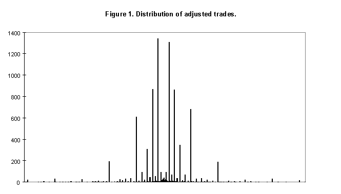
Each transaction record included the transaction price and the quantity traded. Estimation was not carried out using the raw quantity traded data. Rather, the trade quantity was adjusted in three ways. The first adjustment was to reduce the inordinate effect of a handful of extreme outliers. This can be justified by the argument that the technique is best suited to revealing the average effects of typical information trade, rather than infrequent extreme events. It is likely that very extreme trades were negotiated in a way which is not typical and it is also probable that the market maker would have arranged hedging to cover the risk associated with the position taken as a result of these infrequent occurrences. Trades of over IR£50 million of stock were simply cut down to equal IR£51 million. This only affected a handful of trades. At this point it was obvious that even for the truncated quantity data, trades in the range IR£7 million - IR£51 million could be considered atypical or outlying and would be given too much weight in a maximum likelihood estimation framework which assumed normality. To further restrict the effect of outlying observations all trades between IR£7 million and IR£51 million were squeezed linearly and monotonically into the range IR£7 million - IR£20.5 million. The total effect of this set of adjustments gave rise to a distribution as shown in figure (1) below. The standard deviation of the so-far-adjusted trade quantity distribution was roughly IR£5 million. The data was now adjusted further by dividing by IR£5 million. The result was a distribution which was not significantly different in shape from a standard normal distribution. Apart from ensuring that outliers do not dominate the estimation process, another benefit of this standardisation is that it gives rise to coefficients which should have a similar magnitude and this contributes to the ease with which the estimation itself can be achieved.
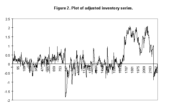
The inventory data was compiled using the cumulated trade data from the truncated stage of adjustment. The cumulative sum was considered to be an indication of the inventory position and this was divided by IR£5 million so that the proportional relation between inventory and the adjusted trade data was almost entirely maintained. A plot of the adjusted inventory series is shown in figure (2) below. Since the inventory begins to appear non-stationary in the last quarter of the available period it was decided to only use data covering the first three quarters. The only other adjustment to the raw data was that the transaction price data was transformed into natural logs and multiplied by 100. This allows for an interpretation of the transitory and permanent price innovation variance in term of percentage returns.
ESTIMATION:
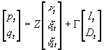
As was mentioned above, the decomposition involved in the implementation of this technique could be achieved by estimating a VMA and using a similar technique to that proposed by Beveridge and Nelson (1981). Of course, a different assumption about the correlation between transitory and permanent innovation would have to be included. Also, the decomposition would have to account for the fact that permanent innovations only enter the transaction price returns since the trade data is stationary. An alternative to this approach is to put the model in state-space form and apply the Kalman filter, taking account of any necessary restrictions during estimation. In fact, the standard-form of the theoretical model is already virtually in state-space form. To make this more explicit we need only add the state equation.
A possible state-space form of the model is;
‘measurement’
![]() (23.1)
(23.1)
‘state’
![]() (23.2)
(23.2)
where, in this case ![]() in the measurement equation, and
in the measurement equation, and ![]() is the transition matrix. For convenience, I use Harvey’s (1989) notation for the variance of transitory and permanent innovations. Thus
is the transition matrix. For convenience, I use Harvey’s (1989) notation for the variance of transitory and permanent innovations. Thus 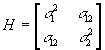 and
and ![]() . In addition the initial value for the state is denoted
. In addition the initial value for the state is denoted ![]() and the initial variance of this is
and the initial variance of this is ![]() , (this notation should not be confused with that used for transaction price
, (this notation should not be confused with that used for transaction price ![]() ).
).
The problem with this common form of the state-space model (23.1-23.2) is that it is not obvious how to include correlation between the permanent and transitory innovations. An alternative representation makes the transitory innovations part of the state equation as follows;
‘measurement’
 (24.1)
‘state’
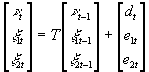 (24.2)
where, in this case;
![]() , and
, and  while,
 ![]() and
and 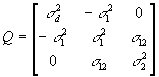 .
.
The exact restriction on the covariance between transitory and permanent innovations implied by the theoretical model is explicitly included in the ![]() matrix.
matrix.
The filter is initialised by providing starting values for the variances of the three innovations and the covariance between the two stationary innovation processes. Initial values for the states must also be provided, (in this case the first state variable is set equal to the transaction price in the first period and the other two states are set equal to zero). Given these initial conditions the filter provides the optimal up-dating of the state variables and the variance parameters. The filter consists of the following equations for each up-dating period;
 (37)
(37)
One problem that often arises in the practical implementation of this filter concerns the maintenance of a positive-definite inverse of ![]() . This condition can eventually fail if bad initial parameters are provided. The condition can be forced as a restriction on the parameters being estimated. This gives rise to new starting values that, if close enough to their unrestricted counterparts, will maintain the inversion condition during the remaining iterations of the unrestricted estimation. This approach was adopted successfully in the application below.
. This condition can eventually fail if bad initial parameters are provided. The condition can be forced as a restriction on the parameters being estimated. This gives rise to new starting values that, if close enough to their unrestricted counterparts, will maintain the inversion condition during the remaining iterations of the unrestricted estimation. This approach was adopted successfully in the application below.
To ensure a sensible application of the theoretical model outlined above it was necessary to introduce an expected trade quantity into the trade equation. Thus, the empirical model that was actually estimated included a parameter ![]() which was multiplied by the trade type indicator so that the matrix
which was multiplied by the trade type indicator so that the matrix ![]() becomes;
becomes;
![]() .
.
This implies that, given knowledge of trade type, the expected trade quantity would not be informative. Finally, it was found necessary to impose the sign restrictions implied by the theoretical model on the parameters of the ![]() matrix. This can be justified purely on theoretical grounds.
matrix. This can be justified purely on theoretical grounds.
IV. RESULTS:
The results from the application of the filter to the data as described above, gave rise to the estimation results contained in table (1) below. The parameter estimates are reasonably precisely estimated with the smallest t-statistic of 6.532. The significant coefficient ![]() indicates that there is an inventory control effect which is positive. This is consistent with a spread which is asymmetrically positioned around the underlying value. The
indicates that there is an inventory control effect which is positive. This is consistent with a spread which is asymmetrically positioned around the underlying value. The ![]() estimate implies that there is a significant order processing cost component which is much larger than the inventory control component. The estimates of the variances of the three signals implies that the private information signal and the signal transmitted by trade have very large imprecision relative to the public information signal. These result in very small Bayesian weights given to the private information signal and as a consequence the trade signal. The weight given to the public signal by the informed trader and the market maker are
estimate implies that there is a significant order processing cost component which is much larger than the inventory control component. The estimates of the variances of the three signals implies that the private information signal and the signal transmitted by trade have very large imprecision relative to the public information signal. These result in very small Bayesian weights given to the private information signal and as a consequence the trade signal. The weight given to the public signal by the informed trader and the market maker are ![]() and
and ![]() respectively. These are both around 0.55. The weight given to the prior of
respectively. These are both around 0.55. The weight given to the prior of ![]() by the informed trader and the market maker are
by the informed trader and the market maker are ![]() and
and ![]() respectively. Since
respectively. Since ![]() and
and ![]() are extremely close to zero the weights are approximately equal to
are extremely close to zero the weights are approximately equal to ![]() and
and ![]() . The actual weights are 0.4397 and 0.441 respectively. Thus, public information is given only slightly more weight than the prior.
. The actual weights are 0.4397 and 0.441 respectively. Thus, public information is given only slightly more weight than the prior.
Diagnostics on the residuals from the two equations of the system do not give rise to concerns over serious miss-specification.
V. SUMMARY AND CONCLUDING COMMENTS:
A new model of Bayesian behaviour was proposed above to improve upon the work of Madhavan and Smidt (1993). A new empirical approach was proposed and implemented in the context of this new theoretical model and gave rise to deeper measures of microstructural characteristics than those available in the existing literature. Specifically, the new approach yields measures of the components that make-up a large number of microstructural parameters. This means that it is possible to talk about the causes of differences in microstructure rather than just describing those differences. The approach was successfully applied to the case of the Irish Gilt-edged securities market and revealed that there is very little adverse selection risk for market makers in this market. This supports evidence for the UK Gilt market produced by Proudman (1995).
It remains to suggest that this approach could be extended both theoretically and in terms of its application. The most obvious theoretical extension would allow prior beliefs to be determined in a recursive fashion by the previous period’s posterior beliefs. This would imply differences in prior beliefs held by the different types of traders. The most obvious empirical extension would be an application to the equity market where it might be more realistic to expect an adverse selection component of trading costs. Apart from these extensions it would be possible to incorporate time variation in the Bayesian weights by use of a stochastic volatility estimation approach. All of these extensions would deepen our understanding of microstructural behaviour in the context of a market making trading environment.
VI APPENDIX (A):
In this appendix the basic steps of the simplification of the equations (19.1-19.3) are shown. Equation (19.1) is reproduced here as (A.1.1)
![]() (A.1.1)
(A.1.1)
A slight restatement of this is;
 (A.1.2)
Now it is easy to show from the construction of Bayesian weights that ![]() can be expressed as follows;
can be expressed as follows;
 (A.1.3)
Notice that ![]() therefore has similarities with the term in the square brackets of equation (A.1.2). This becomes more explicit if we add and subtract
therefore has similarities with the term in the square brackets of equation (A.1.2). This becomes more explicit if we add and subtract ![]() from equation (A.1.2) to get;
from equation (A.1.2) to get;
 .(A.1.4)
Equation (A.1.3) implies that the term in the square brackets can be replaced by
![]() . The result of this is;
. The result of this is;
![]() (A.1.5)
(A.1.5)
or simply the first way of expressing ![]() as shown in equation (20.1) which is;
as shown in equation (20.1) which is; ![]() . The alternative way of expressing this can be found by using the definition of the parameter
. The alternative way of expressing this can be found by using the definition of the parameter ![]() . This is;
. This is;
![]() (A.1.6)
(A.1.6)
Substitution of this way of expressing ![]() gives the alternative expression
gives the alternative expression ![]() .
.
A similar approach was used to simplify the other two equations (19.2) and (19.3). Specifically, the Bayesian weights were re-arranged so that ![]() and
and ![]() could be written entirely in terms of
could be written entirely in terms of ![]() and
and ![]() . Ordinary algebraic manipulation of the resulting expressions gave rise to the simplified versions of equations (19.2) and (19.3) as shown in (20.2) and (20.3) respectively.
. Ordinary algebraic manipulation of the resulting expressions gave rise to the simplified versions of equations (19.2) and (19.3) as shown in (20.2) and (20.3) respectively.
VII. BIBLIOGRAPHY:
Beveridge, S. A. and Nelson, C. (1981). ‘A New Approach to the Decomposition of Economic Time Series into Permanent and Transitory Components with Particular Attention to the Measurement of the Business Cycle’, Journal of Monetary Economics, 7: 151-174.
Blanchard, O., and D. Quah, (1989) "The Dynamic Effects of Aggregate Demand and Supply Disturbances." American Economic Review, Vol. 79., pp 655-673.
Choi, J.Y., Salandro, D. and Shastri, K. (1988). ‘On the Estimation of Bid-Ask Spreads: Theory and Evidence’, Journal of Financial and Quantitative Analysis, 23(2): 219-230.
Copeland, T. E., and Galai, D. (1983). ‘Information Effects on the Bid-ask Spread’, The Journal of Finance, 38(5): 1457-1469.
Dennis and Schnabel, (1983) "Numerical Methods for Unconstrained Optimization and Nonlinear Equations", New Jersey: Prentice-Hall.
Garman, M. (1976). ‘Market Microstructure’, Journal of Financial Economics, 3(1): 257-75.
George, T.J., Kaul, G., and Nimalendran, M. (1991). ‘Estimation of the Bid-Ask Spread and Its Components: A New Approach’, The Review of Financial Studies, 4(4):623-656.
Glosten, L. (1987). ‘Components of the Bid-Ask Spread and the Statistical Properties of Transaction Prices’, Journal of Finance, XLII(5): 1293-1307.
Glosten, L. R., and Milgrom, P. R. (1985). ‘Bid, Ask and Transaction Prices in a Specialist Market With Heterogeneously Informed Traders’, Journal of Financial Economics, 14: 71-100.
Glosten, L. R., and Harris, L. E. (1988). ‘Estimating the Components of the Bid-Ask Spread’, Journal of Financial Economics, 21: 123-142.
Harris, L. (1990). ‘Statistical Properties of the Roll Serial Covariance Bid-Ask Spread Estimator’, The Journal of Finance, XLV(2): 579-590.
Harvey, A.C. (1989), Forecasting, structural time series models and the Kalman filter, Cambridge University Press.
Harvey, A.C. (1997), Messy Time Series: A Unified approach, The Suntory Centre, London School of Economics, Discussion Paper No. EM/97/327.
Hasbrouck, J. (1991a), ‘Measuring the Information Content of Stock Trades’, Journal of Finance, 46(1): 179-207.
--- (1991b). ‘The Summary Informativeness of Stock Trades: An Econometric Analysis’, The Review of Financial Studies, 4: 571-595.
--- (1993). ‘Assessing the Quality of a Security Market: A New Approach to Transaction Cost Measurement’, The Review of Financial Studies, 6(1): 191-212.
Hasbrouck, J., and Ho, T.S.Y. (1987). ‘Order Arrival, Quote Behaviour, and the Return-Generating Process’, Journal of Finance, XLII(4): 1035-48.
Hasbrouck, J., and Sofianos, G, (1993). ‘The Trades of Market Makers: An Empirical Analysis of NYSE Specialists’, Journal of Finance, XLVIII(5): 1565-1593.
Madhavan, A., and Smidt, S. (1991). ‘A Bayesian Model of Intraday Specialist Pricing’, Journal of Financial Economics, 30: 99-134.
Madhavan, A., and Smidt, S. (1993). ‘An Analysis of Changes in Specialist Inventories and Quotations’, Journal of Finance, XLVIII(5): 1595-1628.
Naik, N., and Yadav, P. (1997), ‘Execution costs and Order Flow Characteristics in Dealership Markets: Evidence from the London Stock Exchange’, mimeo, London Business School.
National Treasury Management Agency(1994), Ireland: Proposals for Development of a Market Making System in Government Bonds, Dublin.
O’Hara, M.(1995), Market Microstructure Theory, Cambridge, Mass.
Proudman, J. (1995) "The Microstructure of the UK Gilt Market.", Bank of England Working Paper Series, No. 38.
Roll, R. (1984). ‘A Simple Implicit Measure of the Effective Bid-Ask Spread in an Efficient Market’, Journal of Finance, XXXIX(4): 1127-1139.
Stoll, H. R. (1989). ‘Inferring the Components of the Bib-Ask Spread: Theory and Empirical Tests’, Journal of Finance, XLIV(1): 115-134.
Watson, M. W. (1986). ‘Univariate Detrending Methods with Stochastic Trends’, Journal of Monetary Economics, Vol. 40, pp. 723-739.
Table 1. Results from application to the most frequently traded Gilt-edged security.
|
Parameter |
Estimate |
Standard Error |
T-Statistic |
|
Number of obs. |
2270 |
||
|
Log-Likelihood |
-1139.07 |
||
|
|
0.0804 |
0.0025 |
32.757 |
|
|
0.0686 |
0.0014 |
49.360 |
|
|
0.8290 |
0.0094 |
87.855 |
|
|
-0.0238 |
0.0029 |
-8.024 |
|
|
0.0041 |
0.0006 |
6.532 |
|
|
0.0574 |
0.0030 |
18.731 |
|
|
9.049 |
0.7987 |
11.330 |
|
|
0.0051 |
||
|
|
0.9801 |
||
|
|
1.0729 |
||
|
|
0.00655 |
||
|
|
0.55736 |
||
|
|
0.000004 |
||
|
|
0.55898 |
||