L-scaling

Eric Blankmeyer

Department of Finance and Economics

Southwest Texas State University

San Marcos, TX 78666

512-245-3253

Abstract. This paper introduces L-scaling, which computes

scaled scores from multivariate data. We demonstrate the

uniqueness, positivity, and equivariance of the L-scaling

weights. The relationship of L-scaling to ANOVA and

principal components is explained, robustness and

inference are discussed, and an analogy in mechanics is

mentioned. Finally, L-scaling is used to summarize the cost

of living in 15 U. S. cities in 1988.

Copyright 1996 Eric Blankmeyer

L-scaling

1. Introduction.

This paper introduces L-scaling, a technique for deriving

scaled scores or index numbers from a data matrix. The

weights which L-scaling applies to the data matrix have

several interesting properties:

o they provide a least-squares fit to the data, taking full

account of the correlation matrix;

o they are uniquely defined even if the correlation matrix

does not have full rank;

o they are positive if the correlation matrix is positive;

o they are equivariant with respect to a rescaling of the

data;

o they are related to the principal component method;

o they are also related to the Leontief matrix of economics

(hence the name L-scaling);

o they are easily computed by solving a set of simultaneous

linear equations;

o they can also be computed in a robust form that is

resistant to outliers;

o they have analogues in statistical mechanics and

o they can be used to make inferences and test hypotheses.

The paper is organized as follows. This section defines some

notation. In section 2, the L-scaling weights are shown to be the

unique solution to a least-squares problem. In section 3, the

method's resemblance to the Leontief matrix provides a sufficient

condition for the L-scaling weights to be positive; and

the technique is related to ANOVA and principal components.

Section 4 deals with issues of equivariance and robustness. An

analogy in mechanics is mentioned in section 5, while section 6

addresses inference and hypothesis tests. The paper concludes with an

application to the cost of living in 15 U. S. cities in 1988.

Given T joint observations on K variables, it is frequently

useful to consider the weighted average or scaled score:

In matrix notation,

y = Xw = XWe . (1)

In equation (1),

X = a TxK data matrix to be scaled (the input);

y = a column vector of T scaled scores (the output);

w = a column vector of K weights;

e = a column vector of K units (1's); and

W = a KxK diagonal matrix whose nonzero elements

are the weights (w = We).

To simplify the mathematical notation, it is assumed that the

data have been standardized and divided by the square root of T. That is,

R = X'X (2)

is a correlation matrix of order K. This premise is relaxed in

section 4, where equivariance is discussed. Another assumption is

that the K variables are not all perfectly correlated: the rank

of R exceeds one. In applications, the rank of R is usually the

smaller of T and K since there is unlikely to be an exact linear

relationship among the variables.

2. A least-squares problem.

Because the variables are imperfectly correlated, there are

potentially TK discrepancies between the weighted average y and

its components XW. In view of equation (1), L-scaling defines

such a discrepancy as X_tkw_k - y_t/K. In matrix notation, the TxK

discrepancy matrix is

D = XW - ye'/K

= XW - XWee'/K from (1)

= XW(I - ee'/K) , (3)

where I is the identity matrix of order K. The matrix (I - ee'/K)

is familiar to statisticians; it transforms an array of raw data

into deviations from the sample means. In equation (3), however,

the "data" XW include the observations X and the still unknown

weights W. L-scaling chooses the weights to minimize the sum of

the squared discrepancies. In other words, the weights minimize

the trace (tr) of D'D, just the sum of that matrix's diagonal

elements:

tr(D'D) = tr{[XW(I - ee'/K)]'[XW(I - ee'/K)]}

= tr{XW(I - ee'/K)][XW(I - ee'/K)]'} (4)

since in general tr(PQ) = tr(QP) for conformable matrices.

Moreover, (I - ee'/K) is an idempotent matrix, so equation (4)

becomes

tr(D'D) = tr[XW(I - ee'/K)WX'] . (5)

In equation (5), the diagonal element t of the bracketed

matrix is

where the summations over j and k run from 1 to K. Since the X

data are standardized, it follows from equation (6) that the

L-scaling minimand is

tr(D'D) = w'(I - R/K)w . (7)

To avoid the trivial solution (w = 0), (7) must be minimized

subject to a normalization of the weights. L-scaling adopts the

constraint that the weights should add to 1:

w'e = 1 , (8)

Whether the constrained minimum is unique depends on the rank

of (I - R/K) = (KI - R)/K. The matrix is evidently singular if

and only if K is an eigenvalue of R. But then the rank of R is 1,

contrary to assumption; and the K variables collapse to a single

variable. Barring this, the rank of R exceeds 1, the inverse of

(I - R/K) exists, and the L-scaling minimum is unique. This

conclusion is valid whether or not T > K and even if some (but

not all) of the X variables are linearly dependent.

When the quadratic form (7) is minimized with respect to w

and subject to the normalizing constraint (8), the L-scaling

weights are

w = c(I - R/K) ^-1e (9)

In equation (9), the positive constant

c = 1/e'(I - R/K) ^-1e (10)

is the Lagrange multiplier for the normalizing constraint; it

is also the value of the quadratic form (7) at its constrained

minimum. The scaled scores y are obtained by substituting (9)

into (1).

In many applications of scaling, all the correlations are

positive; in other words, the K variables tend to rise and fall

together. While L-scaling can certainly be applied in other

situations, it will be assumed in this section that R is a

positive matrix.

In that case, the array (I - R/K) bears a formal resemblance

to the Leontief matrix, which figures prominently in the economic

theory of production and growth. Such matrices are positive

definite. Moreover, they have positive elements on the principal

diagonal and negative elements elsewhere. Hawkins and Simon

(1949) and Blankmeyer (1987) show that these properties guarantee

a strictly positive inverse. It follows from equations (9) and

(10) that the L-scaling weights are also strictly positive. In

short, R > 0 is a sufficient condition for w > 0. It is not,

however, a necessary condition, since the L-scaling weights will

often be positive even if some correlations are zero or negative.

In some applications, positive weights are desirable since a

negative weight may be hard to interpret. In section 7, for

example, a cost-of-living index will be computed from several

categories of expenditures. It does not seem obvious what meaning

one would give to a negative weight for an expenditure category.

Waugh (1950) shows that the Leontief inverse can be expanded

in power series. For L-scaling the expansion is, apart from the

factor c,

y = X(I - R/K) ^-1e = Xe + XRe/K + XR²e/K² + ... +

XRⁿe/Kⁿ + ... , (11)

where n is a positive integer. The sequence converges since Re/K

< e.

The first term in the sequence is Xe, just the row totals of

the data matrix. Term n in the sequence approximates the largest

eigenvector of R if n is a large integer. Accordingly, the

L-scaling solution subsumes two well-known scaling techniques:

the one-way analysis of variance (ANOVA) based on row means and

the first principal component of the correlation matrix.

In fact, if the L-scaling quadratic form is minimized on the

unit sphere (w'w = 1) rather than on the plane (w'e = 1), the

first principal-component is obtained. Specifically, the weights

that minimize on the unit sphere

w'(I - R/K)w

= w'w - w'Rw/K

= 1 - w'Rw/K (12)

evidently minimize -w'Rw or equivalently maximize w'Rw.

4. Equivariance and robustness.

Equivariance means that the scaled scores y are unaltered

when a variable in the X matrix undergoes a change of units. This

result follows if the normalization (8) is generalized:

w's = 1 , (13)

where s is the vector of K standard deviations of the variables

in X. The simple sum of the weights has been replaced by the

inner product of the weights and the standard deviations. It is

easy to see how this renormalization achieves equivariance:

whether or not the data have been standardized, the L-scaling

minimand is

When the derivative of (14) with respect to w_k is set equal

to zero,

So w_k is just the coefficient in the (constrained)

least-squares regression of y/K on variable k. Now it is well

known that least-squares regression is equivariant. Suppose that

variable k is rescaled. If each observation X_tk is multiplied by

some positive constant z, its standard deviation s_k is also

multiplied by z. Therefore, in (15) the numerator is multiplied

by z and the denominator is multiplied by z², so w_k is merely

divided by z. It follows from (1) that this change of units has

no effect on the scaled scores y. Accordingly, one may

as well work with the correlation matrix in the first

place, in which case the normalizations (8) and (13) are

identical. Blankmeyer (1994) obtains a similar result for

principal components based on a theorem of Malinvaud (1980, pages

39-42).

If the X matrix may contain outliers, a robust approach is

required. Rousseeuw and Leroy (1987, chapter 7) show how to

compute multivariate means and moment matrices (like R) that are

very resistant to anomalous observations. Their Minimum Volume

Ellipsoid (MVE) is affine equivariant and has a breakdown point

of approximately fifty percent. This means that the estimates are

unaffected by outliers as long as these amount to less than half

the observations.

A limitation of the MVE is its low efficiency at normal

distributions, but there are several ways to deal with that

problem. For example, one can use the MVE to make a preliminary

identification of aberrant data, which can then be discarded,

downweighted, or validated and retained in the sample. Finally,

the familiar least-squares estimates of means and moment matrices

can be applied to the revised data.

Another drawback is the extensive computation required to

estimate the MVE or its variants. Several stand-alone computer

programs are in the public domain at this time (e.g. in Stat.lib

on the Internet). They include Rousseeuw's MINVOL and the

"feasible solution algorithm" of Hawkins (1994). Rocke and Woodruff (1996)

report extensive simulations with MVE and other robust methods; they

also provide a software program.

Farebrother (1987, 1992) has proposed mechanical analogues of

certain statistical techniques including least squares,

orthogonal regression, the L1 norm and the least median of

squares. In this spirit, we remark that the L-scaling matrix

(I - R/K) resembles the "stiffness" matrix, which has a prominent

role in mechanics. Outlining a physical model like Farebrother's,

Strang (1986, 42-44) alludes to the property (I - R/K) ^-1 > 0:

"Positivity means that when all the forces f go in one direction,

so do all the displacements....In the continuous case we will

find the same property for a membrane; when all the forces act

downwards, the displacement is everywhere down." Strang also

comments (tongue in cheek ?) on Leontief matrices in general:

"A matrix with non-positive off-diagonal elements is an

M-matrix if its inverse is nonnegative. No less than 40

equivalent descriptions have been given without assuming

symmetry: all pivots are positive, all real eigenvalues are

positive, and 38 others. With symmetry this means it is positive

definite."

Having discussed L-scaling as a descriptive technique, we

now sketch an inferential model, focusing on the asymptotic

distribution of the scaled scores y when K is fixed. We are interested

in testing hypotheses about the differences in these scores -- say

y_t - y_u . Suppose that the observation matrix X is a random

sample from a multivariate normal distribution with zero mean

vector and correlation matrix R. In large samples, R is

estimated with negligible sampling error; the same is therefore

true of w and c. Equation (1) shows that, asymptotically, the main

cause of sampling variation in y is X itself. In other words, each

element of the y vector is approximately a linear combination of

standard normal variables. Moreover, the elements of y are almost

statistically independent since the only source of correlation among

them is the common weight vector w, and its sampling variation is

minor when T is large. Equation (1) also implies that the variance of each

y element tends to

w'Rw . (16)

Accordingly, an hypothesis that two scaled scores are equal

can be tested by the difference y_t - y_u divided by the square root

of twice (16). If the hypothesis is correct, this statistic has approximately

a standard normal distribution, provided the sample size is large enough.

The preceding analysis is supported by a small simulation study reported

in an appendix to this paper.

7. An example: cost-of-living in U. S. cities.

We now compute a cost-of-living index for 15 U. S.

metropolitan areas in 1988. The exercise is merely intended to

illustrate L-scaling calculations. There is no pretense of

addressing the many difficult research issues that would arise in

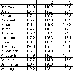
a serious investigation of the topic. Table 1 shows the

three expenditure groups which are to comprise the index. (T = 15

and K = 3).

Table 1. Expenditure groups for selected U. S.

metropolitan areas in 1988 (1982-84 = 100)

(1) food and beverage, (2) apparel and upkeep, (3) entertainment

Source: U. S. Department of Commerce (1990), Tables 698 and 764.

The correlation matrix R is

1.0000 .3150 .2967

.3150 1.0000 -.0036

.2967 -.0036 1.0000

To obtain the L-scaling matrix, we multiply every diagonal

element of R by 1-1/K or 2/3; and we multiply each off-diagonal

element by -1/K or -1/3. The new matrix is then inverted;

(I - R/K)^-1 =

1.5735 .2474 .2330

.2474 1.5389 .0340

.2330 .0340 1.5345

As discussed in section 3, the inverse matrix is positive even

though R is not a positive matrix. The minimized sum of squares

is c = .1762, and each weight is a row sum of c(I - R/K) ^-1. Thus

w' = (.3619, .3207, .3174). When the data in Table 1 are standardized,

the scaled scores y = Xw are shown in the first column of Table 2 below.

Table 2. Cost-of-living indexes for selected U. S.

metropolitan areas, 1988

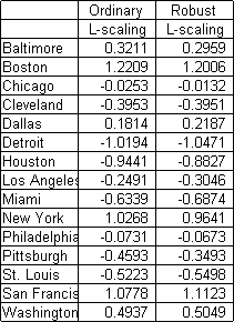
To illustrate an hypothesis test, we ask whether the

cost of living was the same in Boston and Washington DC.

Could the computed difference in column 1 of Table 2 be due to

sampling error ? Although our sample is hardly of the asymptotic

order, we proceed to compute the variance in equation (16); it

is 0.4751, and the square root of twice this number is 0.9748. The

test statistic is therefore (1.2209 - 0.4937)/0.9748 = 0.7459. Considered

as a standard normal variable, this number is not unusually large, so the

hypothesis of equal living costs in Boston and Washington is not rejected

at conventional levels of significance. However, this conclusion is suspect

since the elements of y are unlikely to have the required independent

normal distribution in a sample as small as this one. Incidentally, the

corresponding test statistic for a one-way ANOVA is (1.1970 - 0.5055) /

0.7291 = 0.9484. The two methods, L-scaling and ANOVA, produce

similar y values for Boston and Washington. However, the standard

deviations of the contrasts differ markedly because L-scaling uses

the correlation matrix while ANOVA does not.

To screen for outliers, the MVE was computed with Rousseeuw's

MINVOL program. Taking into account all variables and

observations, the expenditure pattern for Houston is identified as

very anomalous; its robust Mahalanobis distance is quite large.

Dallas and Pittsburgh are flagged as moderately unusual. A

perusal of Table 1 suggests that apparel and upkeep are dispro-

portionately cheap in the Texas cities, while food and beverage

costs are perhaps exceptionally low in Pittsburgh. The correlation

matrix based on the other 12 cities does appear to differ notably

from the full-sample R reported above:

1.0000 .2992 .6332

.2992 1.0000 .5355

.6332 .5355 1.00000

The robust L-scale weights are w' = (0.3291, 0.3137, 0.3572). The

corresponding scores are shown in the second column of Table 2.

To decide whether the two columns differ notably, one should compute

a robust measure of dispersion corresponding to the standard deviation.

The median absolute deviation could be calculated for column 2, or one

could use the more efficient high-breakdown statistics proposed by

Rousseeuw and Croux (1993).

In conclusion, we acknowledge that the literature on scaling

methodology is vast; there is a plethora of techniques for

reducing and describing multivariate data. Our excuse for

introducing still another procedure is that L-scaling has

attractive properties and is related to well known concepts in

statistics, economics, and mechanics.

Blankmeyer, Eric. 1987. "Approaches to Consistency Adjustment."

Journal of Optimization Theory and Applications 54, 479-

488.

Blankmeyer, Eric. 1994. "Principal Components and Scale

Dependence." Paper number TM021242 distributed by the

Educational Resources Information Center (ERIC),

Rockville, MD.

Farebrother, R. W. 1987. "Mechanical Representations of the L1

and L2 Estimation Problems" in Yadolah Dodge (editor)

Statistical Data Analysis Based on the L1-Norm and Related

Methods. Amsterdam: North-Holland.

Farebrother, R. W. 1992. "The Geometrical Foundations of a Class

of Estimation Procedures which Minimise Sums of Euclidean

Distances and Related Quantities" in Yadolah Dodge (editor)

L1-Statistical Analysis and Related Methods. Amsterdam:

North-Holland.

Hawkins, David and Herbert A. Simon. 1949. "Some Conditions of

Macroeconomic Stability." Econometrica 17, 245-48.

Hawkins, Douglas M. 1994. "The feasible solution algorithm for

the minimum covariance determinant estimator in multivariate

data." Computational Statistics and Data Analysis 17, 197-

210.

Malinvaud, Edmond. 1980. Statistical Methods of Econometrics.

Amsterdam: North-Holland.

Rocke, David M. and David L. Woodruff. 1996. "Identification of

Outliers in Multivariate Data." Journal of the American Statistical

Association 91, 1047-1061.

Rousseeuw, Peter J. and Annick M. Leroy. 1987. Robust Regression

and Outlier Detection. New York: Wiley.

Rousseeuw, Peter J. and C. Croux. 1993. "Alternatives to the

Median Absolute Deviation." Journal of the American

Statistical Association 88, 1273-1283.

Strang, Gilbert. 1986. Introduction to Applied Mathematics.

Wellesley: Wellesley-Cambridge Press.

U. S. Department of Commerce. 1990. Statistical Abstract of the

United States 1990. Washington, D. C.: U.S. Government

Printing Office.

Waugh, Frederick. 1950. "Inversion of the Leontief Matrix by

Power Series." Econometrica 18, 142-54.

Appendix: A Simulation of the Large-sample Behavior of y = Xw

The simulation was based on the following correlation matrix R (K = 5):

1.000

0.560 1.000

0.460 0.640 1.000

0.420 0.610 0.730 1.000

0.360 0.520 0.610 0.850 1.000

From equation (16), the asymptotic variance of each element of y is w'Rw. For the correlation matrix listed above, computations show that this variance equals 0.6682. A sample matrix X of one thousand observations (T = 1000) was drawn from a standard normal population with the specified correlation matrix. The weights w and the scaled scores y were computed, and the values for y₂₅₀, y₅₀₀ and y₇₅₀ were saved. This sampling process was replicated 1000 times, and the results were averaged:

Item mean variance

y₂₅₀ 0.0318 0.6858 .

y₅₀₀ 0.0109 0.7237

y₇₅₀ -0.0277 0.6431

The means and variances are therefore close to their theoretical values

(0 and 0.6682 respectively). Moreover, the y values are nearly uncorrelated, as anticipated. The correlations based on 1000 replications were

y₂₅₀ y₅₀₀ y₇₅₀

y₂₅₀ 1.000

y₅₀₀ 0.044 1.000

y₇₅₀ 0.046 0.015 1.000

To examine the normality of the y values, each series of 1000 replications was standardized and its percentiles were computed:

Percentiles of Y₂₅₀:

Minimum -3.1349662272 Maximum 3.3868069221

01-%ile -2.2635771008 99-%ile 2.3000997935

05-%ile -1.6510098850 95-%ile 1.6331218076

10-%ile -1.2789133398 90-%ile 1.2353421952

25-%ile -0.6520738257 75-%ile 0.6665215838

Median 0.0195509971

Percentiles of Y₅₀₀:

Minimum -3.4518302265 Maximum 3.1892254907

01-%ile -2.1820584643 99-%ile 2.4140492365

05-%ile -1.7077252083 95-%ile 1.6806021486

10-%ile -1.2650296564 90-%ile 1.2651179280

25-%ile -0.6577554324 75-%ile 0.6353784205

Median 0.0092066145

Percentiles of Y₇₅₀:

Minimum -3.9126888937 Maximum 3.1864460451

01-%ile -2.3735735447 99-%ile 2.1743808876

05-%ile -1.7210294044 95-%ile 1.5796671591

10-%ile -1.2780010879 90-%ile 1.2595918021

25-%ile -0.6944575422 75-%ile 0.7064393966

Median 0.0140574363

In general, these percentiles are consistent with the theory that each element of y is asymptotically a normal random variable.

Next, the sample size was reduced to T = 100, and 1000 replications were run with the following results:

Item mean variance

y₂₅ -0.0016 0.7026

y₅₀ 0.0240 0.7060

y₇₅ -0.0045 0.6772

The correlations were:

y₂₅ y₅₀ y₇₅

y₂₅ 1.000

y₅₀ -0.008 1.000

y₇₅ -0.004 -0.058 1.000

The percentiles are shown below.

Percentiles of y₂₅:

Minimum -3.0641586435 Maximum 3.2054790509

01-%ile -2.2607769141 99-%ile 2.3173970833

05-%ile -1.6269838530 95-%ile 1.6801338613

10-%ile -1.2594787954 90-%ile 1.3307414199

25-%ile -0.6945332370 75-%ile 0.6722215321

Median -0.0420984134

Percentiles of y₅₀:

Minimum -2.8748829280 Maximum 3.0130409170

01-%ile -2.1936201853 99-%ile 2.1782654350

05-%ile -1.6517804725 95-%ile 1.6606397887

10-%ile -1.2564622698 90-%ile 1.3072116491

25-%ile -0.7231219330 75-%ile 0.7012371942

Median 0.0085705466

Percentiles of y₇₅:

Minimum -2.9664948228 Maximum 2.8521610229

01-%ile -2.2572829258 99-%ile 2.2654368354

05-%ile -1.6413530153 95-%ile 1.6527581800

10-%ile -1.2818094175 90-%ile 1.3387785164

25-%ile -0.6600528320 75-%ile 0.6556602800

Median -0.0043668779

Despite the smaller sample size, these results also appear to be broadly in agreement with our analysis of the asymptotic behavior of the scaled scores.

The preceding conclusions could be made more formal by the application of standard statistical tests. For example, procedures for testing the mean and the variance of a normal distribution are well known (Morrison 1967, 21-28), while the independence of the elements of y can be examined with a chi-square statistic computed from the determinant of the relevant correlation matrix (Morrison 1967, 111-114). Moreover, the normality of each y element could be investigated via a Kolmogorov-Smirnov test (Siegel 47-52).

Morrison, Donald F. (1967). Multivariate Statistical Methods. New York:

McGraw-Hill.

Siegel, Sidney (1956). Nonparametric Statistics for the Behavioral

Sciences. New York: McGraw-Hill.