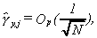
 1 (2.1)
Real and Spurious Long Memory Properties
of Stock Market Data
I.N. Lobato and N.E. Savin
Department of Economics
University of Iowa
Iowa City
IA 52242
Abstract
We test for the presence of long memory in daily stock returns and their squares using a robust semiparametric procedure. Spurious results can be produced by nonstationarity and aggregation. We address these problems by analyzing subperiods of returns and using individual stocks. The test results show no evidence of long memory in the returns. By contrast, there is strong evidence in the squared returns.
KEY WORDS: Long Range Dependence; Semiparametric Procedure; Lagrange Multiplier Test
1. INTRODUCTION
There have been several papers analyzing the long term properties of stock returns. Greene and Fielitz (1977) used the R/S statistic (Hurst (1951)) to test for long term dependence in the daily returns of 200 individual stocks on the NYSE from December 23, 1963 to November 29, 1968 and claim to have found significant evidence. Lo (1991) criticized these results on the grounds that this evidence was due to short term correlation. He proposed a modified version of the R/S statistic to test robustly for long term dependence, and found no evidence in favor of long run dependence of the monthly and daily returns on CRSP stock indices. Ding et al. (1993) examined the long memory properties of several transformations of the absolute value of daily returns on the S&P 500, including squared returns, and found considerable evidence of long memory in the squared returns, but conducted no formal test.
The purpose of this paper is twofold. The first is to conduct a formal test using a semiparametric procedure due to Lobato and Robinson (1996). The null hypothesis is that of weak dependence or short memory, the alternative being strong dependence or long memory. The procedure focuses on the long memory properties of the data irrespective of the short term dependence. Although the R/S procedures are robust, their efficiency properties are questionable; see Robinson (1994). Furthermore, the test statistic used by Lo has a complicated asymptotic distribution when the null is true whereas the test statistic we consider has the convenient feature that its asymptotic distribution is chi-square. Our test accepts weak dependence for daily returns on the S&P 500, but rejects for squared returns. The rejection is even stronger for absolute returns.
The second purpose is to investigate whether rejection of weak dependence is due to long memory or is due to other causes. Two common causes of spurious long memory are nonstationarity and aggregation. Nonstationarity is a plausible explanation for our findings and especially that of Ding et al., who use S&P 500 data from 1928 to 1992. During this period, there were changes in the mean of squared returns. It was very high in the early thirties and then was much reduced by the end of the decade. During the mid seventies and the eighties, there has been a substantial increase in the mean of the squared returns, perhaps due to factors such as the introduction of new financial products and the widespread use of computer trading programs; see, for example, Grossman and Zhou (1996). The mean of squared returns appears to have decreased again in the nineties. Changes in the mean of squared returns also occur for individual stocks.
In the case of stock indices the evidence in favor of long memory may be due to the effect of aggregation. The key idea is that aggregation of independent weakly dependent series can produce a strong dependent series. For example, in the case of the squares of the daily returns of the S&P 500 it could happen that squares for the individual stocks do not exhibit long memory and the apparent long memory of the index is just due to aggregation. A motivation for this can be found, for instance, in Robinson (1978) or Granger (1980).
We address the nonstationarity problem by splitting up the daily data into arguably stationary periods and the aggregation problem by using daily data on the individual stocks in the Dow Jones Industrial Average. Our conclusions confirm the results of Ding et al. (1993). In particular, for subseries of the S&P 500 index that appear stationary our test favors long memory. Similar results are obtained for the subseries for the individual stocks in the Dow Jones Industrial Average.
The organization of the paper
is the following. In Section 2 we briefly review the concept of
long memory and describe the procedure we use to test for long
memory. Section 3 contains our analysis of the long memory properties
of the data. In Section 4 we discuss our results and comment on
intradaily stock returns.
2. TEST STATISTIC
In this section we describe the test statistic that we employ to analyze the long memory properties of the data.
There is no unique definition of a long memory process. Consider a covariance stationary process xt and assume its spectral density function exists and call it f(l). The condition
1 (2.1)
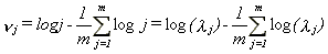
for H<1, H¹1/2, with C a positive constant, characterizes xt as a long memory process. Notice that (2.1) includes two different cases. For HÎ(1/2,1) f(l) tends to infinity as it is evaluated at frequencies that tend to zero (this is called the strictly long memory case) while when H<1/2 it tends to zero (this is called the antipersistent case). The case H=1/2 represents the weakly dependent case; f(l) tends to a constant as it is evaluated at frequencies that tend to zero.
In the time domain, long memory can be characterized as follows. Let gj denote the autocovariance at lag j of xt, gj=E[(x1-m)(x1+j-m)] with m denoting the mean of the process xt. The condition
 2 (2.2)
where K is a constant and H takes the same values as above, characterizes xt as a long memory process.
Conditions (2.1) and (2.2) are not necessarily equivalent, but for fractional ARIMA processes both hold. Notice that when HÎ(1/2,1) both conditions (2.1) and (2.2) imply
 3 (2.3)
This condition is a more general definition of strictly long memory.
H is the parameter that determines the degree of long memory (the higher the H the longer the memory) and so testing the null hypothesis of weak dependence against the alternative of long memory is equivalent to testing H=1/2 against H¹1/2.
Notice that (2.1) only characterizes the behavior of f(l) in a neighborhood of zero and nothing is specified about the medium or short term behavior of the process. Therefore, robust estimation and testing procedures in the frequency domain can be carried out using the periodogram (or some functions of the periodogram) evaluated in a degenerating neighborhood of zero frequency. In order to do so it is necessary to introduce a bandwidth number m that tends to infinity as the sample size (n) tends to infinity, but slowly so that m/n tends to zero.
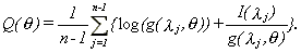
Robinson (1995) analyzed a robust estimation procedure based on the following objective function (see also Künsch, 1987)
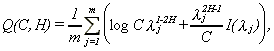 4 (2.4)
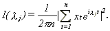
where I(lj) is the periodogram at frequency lj (=2pj/n),
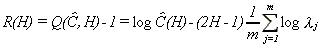
Robinson analyzes the properties of the estimate that minimizes (2.4) in a compact set [D1, D2] with 0<D1<D2<1. Denoting this estimate by _, he proves that
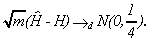 6 (2.5)
This estimate appears to be the most efficient semiparametric estimate developed so far.
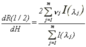
We employ an approximation to the Lagrange Multiplier test to test H=1/2 against H¹1/2 (or H>1/2) based on the objective function (2.4). This test (denoted by LM) is a particular case of the more general test analyzed in Lobato and Robinson (1996). For the univariate case and a two-sided alternative hypothesis, the LM test statistic has the form
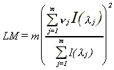 7
(2.6)
7
(2.6)
where
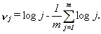 8
8
The details of the objective function and the testing procedure are given in Appendix A. In Lobato and Robinson (1996) conditions are provided which establish under the null hypothesis (H=1/2), that LM®d c12 and also conditions for the consistency of the test. Monte Carlo analysis of this test is also provided. An alternative procedure that sometimes produces slightly better finite sample performance is to use the periodogram of tapered rather than observed data in expression (2.6).
The Wald test can also be based
on (2.4). The disadvantage of the Wald test is that it needs an
estimate for H and so, the minimization of (2.4) has to be carried
out by iterative procedures. Monte Carlo analysis of this test
is reported in Robinson (1995).
3. EMPIRICAL RESULTS
In Table 1 we report results for the LM test of long memory for daily returns, squared returns and the absolute value of the returns for the S&P 500 index between July 1962 to December 1994. The sample size is n=8178. We report the test for a grid of values of m from m=30 to m=100. When m equals 30 and 100, the shortest periods that are taken into account by the test correspond to approximately 273 and 82 days, respectively. No evidence of long memory is found in the returns, but there is strong evidence of long memory in the squares. This evidence is even stronger for the absolute value of the returns and hence we concentrate on the squares. These results are in agreement with Lo (1991) and Ding et al. (1993).
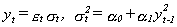
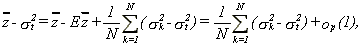
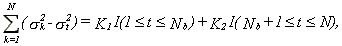
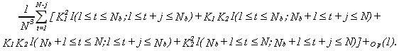
There are several ways in which the LM test for long memory can produce spurious results. First, the squared returns process could posses a shift in the mean. To show how this can happen consider the following set up. Let yt, t=1,2,....N, be a zero mean stochastic process with
9
where yt is independent of ys for t¹s and, for some v>0, Eyt2+v<¥ for all t. Denote the sample autocovariances for y or y2 by
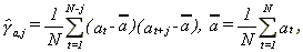 10
10
for j=1,...,N-1, and a=y or y2.
Obviously yt and yt2 are not covariance stationary processes. Hence, the definitions of long memory stated in section 2 do not apply. Nevertheless imagine that the researcher does not know this and tests for evidence of long memory in yt and yt2. What would she find? First consider the behavior of the sample autocovariances for yt. It is immediate to show that
 11
11
for all j, exactly the same as we get with a white noise process and so long memory should not be detected. What about yt2? In Appendix B it is shown that for some constants cj different from zero
 12
12
for all j. So it is not that the sample autocovariances tend slowly to zero. In fact, they do not even tend to zero.
Nonstationarity may be responsible for the findings of Ding et al. (1993). They analyze the S&P 500 series from 1928 to 1992. During this period there are several reasons to suspect nonstationarity. The squared returns appear to be much larger in the thirties than in later periods. The functioning of the stock market may have been affected by World War II. Recently, during the mid seventies and specially the eighties, financial markets have seen the introduction of new financial products and a widespread use of information technology in the trading process. These considerations may be relevant to understand the Ding et al. (1993) results. Our sample goes from July 1962 to December 1994 and so it also covers a period in which the introduction of financial innovations raises questions about the stationarity assumption. To investigate the possibility that the observed evidence of long memory is, in fact, due to nonstationarity, we split our sample into two periods. We take January 1973 as the break point since the oil price shock occured in that year. In Table 1 we present the results of the LM test for long memory for the two subsamples using several values for m. In Figure 1 we plot S&P 500 returns for periods July 1962-December 1972, January 1973-December 1986 and January 1987-December 1994. From this plot there is very clear increase in volatility between the first two periods. The crash in October 1987 dominates the bottom part of Figure 1. Our eyeball test says that the series is stationary during the period 1962-1972 and it may be for 1973-1994. Thus, it is of interest that the squared returns exhibit strong evidence of long memory for the period 1962-1972 as well as for 1973-1994. To our knowledge, no formal test is available for structural change in the mean in the presence of long memory when the time series is not Gaussian (the fact that stock returns are non Gaussian has been established in several papers, see for instance Brock and de Lima, 1995).
The second reason why the evidence of long memory in the squared returns in the S&P 500 can be spurious is based on aggregation. The S&P 500 is an aggregate index of the stock market and so its squared returns are derived from the squared returns of the individual stocks. It may well happen that the specific stocks do not exhibit strong dependence and the apparent long memory of the index is just due to aggregation. A motivation of this can be found, for instance, in Robinson (1978) or Granger (1980). In these papers it is shown that starting with individual independent AR(1) series with random autoregressive coefficients, the aggregate series can exhibit long memory for certain specifications of the distribution function from which these coefficients are drawn. This result can be generalized to other weak dependent processes, in particular ARMA processes. The key idea is that aggregation of independent weakly dependent series can produce a strongly dependent series. In our case, it seems very implausible to assume independence of the squared returns processes for the individual stocks. And so the aggregation explanation in Robinson (1978) and Granger (1980) is not directly applicable. Nonetheless, what is clear is that aggregation may produce spurious evidence of long memory.
To examine this possibility, we analyzed the long memory properties of the thirty stocks which compose the Dow Jones Industrial Average. These thirty stocks are listed in Table 2 with their ticks and periods covered. Except for three cases, the data are for July 1962 to December 1994. These data are taken from the CRSP files. In Tables 3 and 4 we report the LM statistics for the returns and the squared returns for the periods July 1962 to December 1972 and January 1973 to December 1994.
There are several features which should be noticed. First, there is no evidence of long memory in the returns for any period. Second, with respect to the squares the evidence is more varied. For the period July 1962 to December 1972 all stocks but six (ATT, GM, MRK, JPM, S, WX) show strong evidence. For the period January 1973 to December 1994 there is stronger evidence of long memory in the squared returns. It is worth mentioning that the period 1973-1994 has gone through substantial changes in both financial instruments and information technology tools. Thus it is plausible that the squared returns are nonstationary in this period. This could explain the widespread finding of long memory in the squared returns in this period.
The results for the LM test for the whole period are in Table 5. It is not surprising that for all the series there is evidence of long memory in the squared returns. For some stocks, in particular the six noted above, this evidence of long memory may be spurious and may be due to nonstationarity during the whole period.
Nonstationarity and aggregation are two important causes of spurious evidence of long memory but they are not the only ones. In the rest of the section we mention three additional causes.
The third cause is a seasonal long memory component in the returns. This case is analyzed in Lobato (1996). For an exchange rate series (British pound against Deutsche mark for 1989 to 1994) it is shown how the presence of a strong cyclic component of about two weeks in their returns can produce spurious evidence of long memory in the squared returns. However, for the S&P 500 this explanation does not seem applicable.
The fourth cause involves size distortions. In Lobato and Robinson (1996) it is shown that the LM test suffers from severe size distortions in the AR(1) case when the autoregressive coefficient takes values near one, the closer to one the greater the distortion. In Table 6 we report a Monte Carlo study to demonstrate this possibility. We generate 5000 replications of an ARCH(1) process
 13 (3.1)
with sample size=1000, a0=0.1, five values for a1 (0.0,0.3,0.6,0.9,0.95), and where et is independently and identically distributed N(0,1). We consider three values for m, 40,70 and 100, and report the percentage of rejections based on the 5% and 1% critical values of c12. There is some spurious evidence of long memory for a1=0.9 and 0.95 when m=100. When m is smaller, this phenomenon is not so marked. Notice that if ½a1½>1/Ö3, the fourth moment is not finite. In this case our test procedure does not work.
The fifth cause is the nonexistence
of higher order moments. This is motivated by the above comment
on the existence of the fourth moment. The LM test, as well as
the Wald test, for long memory assume that the examined series
has a finite fourth moment. Loretan and Phillips (1993) have argued
that the fourth moment may not exist for financial series. However,
we do not know of a robust test for the nonexistence of moments
in a long memory environment. A robust procedure analyzed in Hsing
(1991) is valid for weak dependent but not for long memory processes.
At any rate, there is no consensus in this matter. For different
series, different results have been found; see, Brock and de Lima
(1995).
4. DISCUSSION
In this paper we have examined the presence of long memory in daily stock returns and their squares using a semiparametric procedure that is robust to the presence of weak dependence. Our test results indicate no evidence of long memory in the levels of the returns. For the squared returns, however, the test results favor long memory and hence confirm the conclusion of Ding et al. (1993). Furthermore, our analysis suggests that this evidence in favor of long memory is real, not spurious.
If there is indeed long memory in the squares of the returns, then the standard statistical tools for inference are not valid (see, for instance, Chapter 1 in Beran, 1994). In particular, inferences about squared returns and volatility using standard techniques can be misleading. For instance, the standard errors for the estimates of the coefficients of conventional ARCH or stochastic volatility models will be incorrect and hence the confidence intervals for predictions.
In the case of long memory in squared stock returns, dependence in stock returns is not properly measured by autocorrelations. However, in the case of the S&P 500, the Box and Ljiung modified Q test statistic does detect dependence when using a small number of lags; this is due to the first autocorrelation. In other cases more refined tests of independence than those based on the spectrum may be needed (see, for instance, Robinson (1991), Skaug and Tjøstheim (1993), Delgado (1996), Pinkse (1996) and references therein).
We also investigated intradaily
stock returns for long memory since these data are now commonly
used in finance (Stoll and Whaley (1990)). In particular, we tested
the minute by minute returns and their squares for IBM, one of
the most heavily traded stocks. The results showed no evidence
of long memory in the returns, but strong evidence for the squared
returns. In this paper, however, we do not present our findings.
The reason is that nonstationarity poses a serious problem in
the case of intradaily returns. It is a well known institutional
fact that intradaily squared returns are nonstationary. For a
period of a day, the time series of intradaily squared returns
has an inverse J shape (Brock and Kleidon (1992) and Madhavan
et al. (1994)). Splitting the intradaily data into what appear
to be stationarity periods does not permit us to test for long
memory because the stationary periods are too short for the distribution
of the test statistic we employ to be well approximated by its
asymptotic normal distribution. One approach to treating the small
sample problem is to patch days together omitting, say, the first
ten minutes of each day; see, for example, Stoll and Whaley (1990).
It is highly questionable whether this is a satisfactory solution
to the nonstationary problem.
ACKNOWLEDGEMENTS: We thank J.
Cotter, D. Foster, N. Kocherlakota, A. Vijh, P. Weller, H. White,
the coeditor, an associate editor and two referees for useful
comments, M.A. Delgado and H. Skaug for the use of their computer
programs and Yue Yu for assistance with the data.
APPENDIX A
To motivate the objective function (2.4) consider the following frequency domain version of the Whittle Gaussian negative log-likelihood for the model f(l)=g(l,q), -p<l£p
 14
14
Expression (2.4) is obtained by assuming that the spectral density function behaves as (2.1) and considering only frequencies close to zero (that is, from l1 to lm).
To motivate the approximate Lagrange multiplier statistic (2.6), first concentrate C out of (2.4), see Robinson (1995, section 2), to get
 15
15
where
 16
16
This implies that the Lagrange multiplier test statistic is
 17
17
Now it is straightforward using Robinson (1995, section 4) to get
 18
18
and
 19
19
Therefore, under the null hypothesis (H=1/2) noticing that
 20
20
we obtain
 21
21
and using Robinson (1995, section 4)
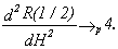 22
22
Therefore an approximate Lagrange
multiplier test statistic is given by (2.6).
APPENDIX B
For simplicity, call zt=yt2 and _ to its mean. Now as zt-st2 is a uniformly integrable zero mean independent sequence, we can apply a Weak Law of Large Numbers (WLLN) to that sequence so that
 23 (A.1)
Now using that
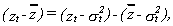 24
24
we get
 25 (A.2)
Now as
 26
(A.3)
26
(A.3)
the last term in (A.2) is
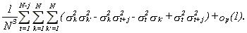 27
27
Furthermore,
 28
28
where K1 and K2 are given by
 29
29
and I(A) is the indicator function, i.e., I(A)=1 if A is true, I(A)=0 otherwise. Then the last term of (A.2) is
 30
30
The first summand is K12(Nb-j) I(j£Nb), the third is zero, the fourth is K22(N-Nb-j)I(j£N-Nb)
and the second is
31
so that the last term in (A.2) tends to a different value depending on j. For 1£j£Nb it is
 32
32
for Nb<j£N-Nb it is
 33
33
and for N-Nb<j£N-1 it is
 34
34
with y=(s22-s12)
and q=Nb/N.
Now the first term in (A.2) is op(1) applying a WLLN
to the uniformly integrable zero mean independent sequence (zt-st2)(zt+j-st+j2)
and the second and third terms are op(1) using (A.1)
and (A.3).
Beran, J. (1994), Statistics for Long-Memory Processes, Chapman & Hall, New York.
Brock, W.A., and Kleidon, A.W. (1992), "Periodic Market Closure and Trading Volume",
Journal of Economic Dynamics and Control, 16, 451-489.
Brock, W.A., and de Lima, P.J.F. (1995), "Nonlinear Time Series, Complexity Theory, and Finance",
Preprint, Social Systems Research Institute, University of Wisconsin-Madison.
Delgado, M.A. (1996), "Testing Serial Independence Using the Sample Distribution Function", forthcoming in Journal of Time Series Analysis.
Ding, Z., Granger C.W.J., and Engle, R.F. (1993), "A Long Memory Property of Stock Returns and a New Model", Journal of Empirical Finance, 1, 83-106.
Granger, C.W.J. (1980), "Long Memory Relationships and the Aggregation of Dynamic Models",
Journal of Econometrics,14,227-238.
Greene, M., and Fielitz, B. (1977), "Long Term Dependence in Common Stock Returns", Journal of Financial Economics, 4, 339-349.
Grossman, S.J. and Zhou, Z. (1996), " Equilibrium Analysis of Portfolio Insurance", Journal of Finance, \ 51, 1379-1403.
Hidalgo, J., and Robinson, P.M. (1996), "Testing for Structural Change in a Long-Memory Environment", Journal of Econometrics, 70, 159-174.
Hsing, T. (1991), "On Tail Index Estimation Using Dependent Data", Annals of Statistics, 19, 1547-1569.
Hurst, H.E. (1951), "Long-Term Storage Capacity of Reservoirs", Transactions of the American Society of Civil Engineers, 116, 770-799.
Künsch, H.R. (1987), "Statistical aspects of self-similar processes", Proceedings of the First World Congress of the Bernouilli Society (Yu. prohorov and V.V. Sazanov, eds.), 1, 67-74, VNU Science Press, Utrecht.
Lo, A.W. (1991), "Long Term Memory in Stock Market Prices", Econometrica, 59, 1279-1313.
Lobato, I. (1996), "An Application of Semiparametric Estimation in Long Memory Models", forthcoming
in Investigaciones Económicas.
Lobato, I., and Robinson, P.M. (1996), "A Nonparametric Test for I(0)", Preprint, Department of Economics, University of Iowa, Iowa City, IA 52242.
Loretan, M., and Phillips, P.C.B. (1993), "Testing the Covariance Stationarity of Heavy-Tailed Time Series:
an Overview of the Theory with Applications to Several Financial Datasets", Journal of Empirical Finance, 1, 211-248.
Madhavan, A., Richardson, M., and Roomans, M. (1994), "Why Do Security Prices Change? A
Transaction-Level Analysis of NYSE Stocks", Preprint, Wharton School, University of Pennsylvania.
Pinkse, C.A.P. (1996), "A Consistent Nonparametric Test for Serial Independence", forthcoming in Journal of Econometrics.
Robinson, P.M. (1978), "Statistical Inference for a Random Coefficient Autoregressive Model", Scandinavian Journal of Statistics, 5, 163-168.
--------(1991), "Consistent nonparametric entropy based testing', Review of Economic Studies, 58, 437-453.
--------(1994), "Time Series with Strong Dependence", In Advances in Econometrics. Sixth World Congress, vol.1 (C.A. Sims, Ed.). Cambridge University Press, pp. 47-95.
--------(1995), "Gaussian Semiparametric Estimation of Long Range Dependence", Annals of Statistics, 23, 1630-1661.
Skaug, H., and Tjøstheim, D. (1993), "A Nonparametric Test of Serial Independence Based on the Empirical Distribution Function", Biometrika, 80, 591-602.
Stoll, H.R., and Whaley, R.E. (1990),
"The Dynamics of Stock Index and Stock Index Futures Returns",
Journal of Financial and Quantitative Analysis, 25, 4,
441-468.
| Series | 30 | 40 | 50 | 60 | 70 | 80 | 90 | 100 |
| Returns | 0.76 | 0.11 | 0.02 | 0.15 | 0.07 | 0.14 | 0.12 | 0.24 |
| Squared returns | 2.50 | 3.68 | 5.06* | 6.14* | 7.60* | 10.3* | 13.5* | 17.0* |
| Absolute value
of returns | 21.8* | 34.6* | 45.6* | 57.3* | 74.4* | 96.5* | 120* | 150* |
| Returns | 0.00 | 0.21 | 0.00 | 0.00 | ||||
| Squared returns | 4.61* | 9.00* | 14.9* | 23.8* | ||||
| Absolute value
of returns | 12.9* | 22.3* | 34.4* | 51.0* | ||||
| Returns | ||||||||
| Squared returns | ||||||||
| Absolute value
of returns | ||||||||
NOTE: * indicates significant at the 5% level. Table 6. LM Percentage of rejections.
|
| |||||||
NOTE: Series follow ARCH(1) as stated in equation (3.1). Sample size=1000.
Number of replications=5000.